7. Run a PERMANOVA

• Overview
• A three-factor hierarchical design
• Steps in a PERMANOVA analysis
• Step 1: Data selection
• Step 2: Jaccard resemblance
• Step 3: Specify the design
• Step 4: Run PERMANOVA
• Step 4 (continued): Key additional details about PERMANOVA in PRIMER
• Step 5: Ordination of centroids
• Summary of the PERMANOVA analysis

Overview

If you have purchased the PERMANOVA+ add-on, then you will have an additional menu item that allows you to perform a broad range of additional analyses using a suite of routines that are not available in the base PRIMER 7 package, including PERMANOVA, PERMDISP, PCO, DISTLM/dbRDA and CAP. See the PERMANOVA+ user manual for details regarding these routines and the underlying methods.

Here, we will run through a quick example of how to set up and run a multi-factor PERMANOVA analysis in PRIMER. Permutational multivariate analysis of variance (PERMANOVA) partitions variation in the space of a chosen dissimilarity measure in response to one or more factors in a specified sampling protocol or experimental design ( Anderson (2001a) , Anderson (2017) ). Tests of individual terms in a PERMANOVA model are achieved by constructing correct (pseudo-)F ratios on the basis of expectations of mean squares (EMS), and p-values are obtained using correct permutation algorithms given the full study design.

Importantly, the PERMANOVA routine in PRIMER allows the user:

• to specify whether factors are fixed or random,
• to specify whether a factor is nested in one or more other factors,
• to test interaction terms,
• to include one or more quantitative covariates in the analysis,
• to remove individual terms from a model or to perform pooling,
• to handle correctly:
  • mixed models
  • user-specified contrasts
  • BACI designs (before-after/control-impact),
  • asymmetrical designs (e.g., in environmental impact studies),
  • randomised blocks,
  • split plots,
  • hierarchical designs,
  • repeated measures,
  • unbalanced designs (Type I, II or III sums of squares),
  • ... and more.

A three-factor hierarchical design

We will run PERMANOVA on an example dataset consisting of assemblages of molluscs collected from holdfasts of the kelp Ecklonia radiata in a 3-factor hierarchical experimental design. There were n = 5 holdfasts collected from each of 2 areas (tens of meters apart) at each of 2 sites (hundreds of meters to kilometers apart) from each of 4 locations (hundreds of kilometers apart) in rocky reef habitats along the northeastern coast of New Zealand ( Anderson et al. (2005a) , Anderson et al. (2005b) ).

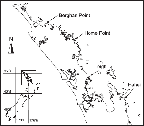
The map above shows the four locations on the northeastern coast of New Zealand from which holdfasts were collected for the study: Berghan Point, Home Point, Leigh and Hahei (reproduced from Fig. 1 in Anderson et al. (2005a) ).

The example data are found in the file called NZ holdfast fauna abundance.pri in the folder named 'NZ holdfast fauna' inside the 'Examples v7' folder that can be downloaded by clicking Help > Get Examples V7.... There were 351 taxa (rows) from 15 different phyla quantified in this study. Here, we shall focus only on the phylum Mollusca (105 taxa).

Our interest lies in quantifying the degree of turnover in the identities of mollusc species at different spatial scales, as measured by the Jaccard resemblance measure. This a fully hierarchical sampling design with three spatial factors, as follows:

• Locations (random with 4 levels: Berghan Point, Home Point, Leigh and Hahei)
• Sites (random and nested in Locations, with 2 sites per location)
• Areas (random and nested in Sites, with 2 areas per site)

Areas are therefore also (necessarily) nested in Locations as well.

Steps in a PERMANOVA analysis

The two essential steps required to run a PERMANOVA analysis in PRIMER are always:

• first, specify the design; and
• then, run the PERMANOVA analysis, given the design, on a chosen resemblance matrix (arising from the data of interest).

Generally, we first need to get our data in to PRIMER, perform appropriate pre-treatment(s), if any, then calculate a resemblance matrix from this. A resemblance matrix will always serve as the starting point for any PERMANOVA analysis.

An analysis of only the mollusc species from the holdfasts in accordance with the three-factor hierarchical design, based on Jaccard resemblances, will follow the following steps:

1. Open the example data file in the PRIMER workspace. Select a subset of the variables corresponding to only the mollusc species for what follows.
2. Calculate Jaccard similarities* among the sampling units (individual holdfasts).
3. Specify the experimental/sampling design (creating a design file).
4. Run the PERMANOVA routine (partitioning and p-values via permutation for each term in the model.
5. Do an ordination of distances among centroids to visualise the effects and the relative importance of the factors.

(*Note: the Jaccard resemblance measure utilises only presence/absence information, so we do not need to perform a pre-treatment transformation step for this example.)

Step 1: Data selection

Open up the example data file

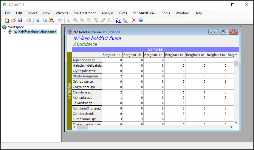
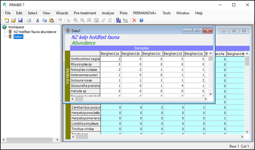
Launch PRIMER, then click File > Open... from the main menu, navigate to the folder named 'NZ holdfast fauna' in the 'Examples v7' directory, and select 'NZ holdfast fauna abundance.pri'. Click Open to display the species matrix.

Click on Edit > Indicators... and you will see that the data includes information about whether individual taxa were counted (enumerated) or quantified on an ordinal scale ('Ordinal' = 'N' or 'Y', respectively). Also shown are indicators showing the taxonomic groups in which each species (or taxon) variable belongs, with different levels of the taxonomic hierarchy being provided as different indicators (i.e., 'Genus', 'Family', 'Order', 'Class' and 'Phylum').

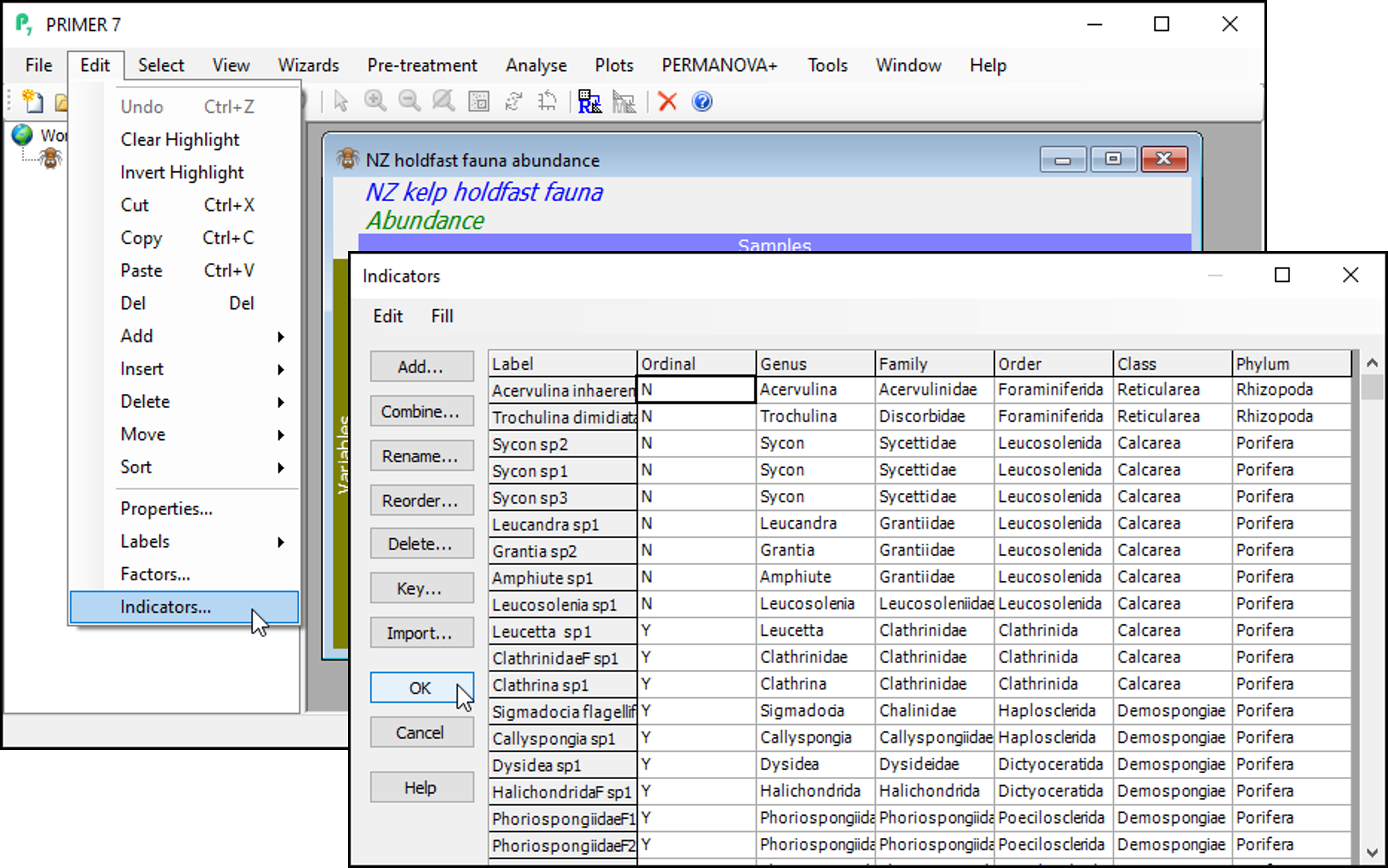
Click OK on the 'Indicators' dialog, so the data matrix is the active item in the workspace again.

Select a subset of variables, using an indicator

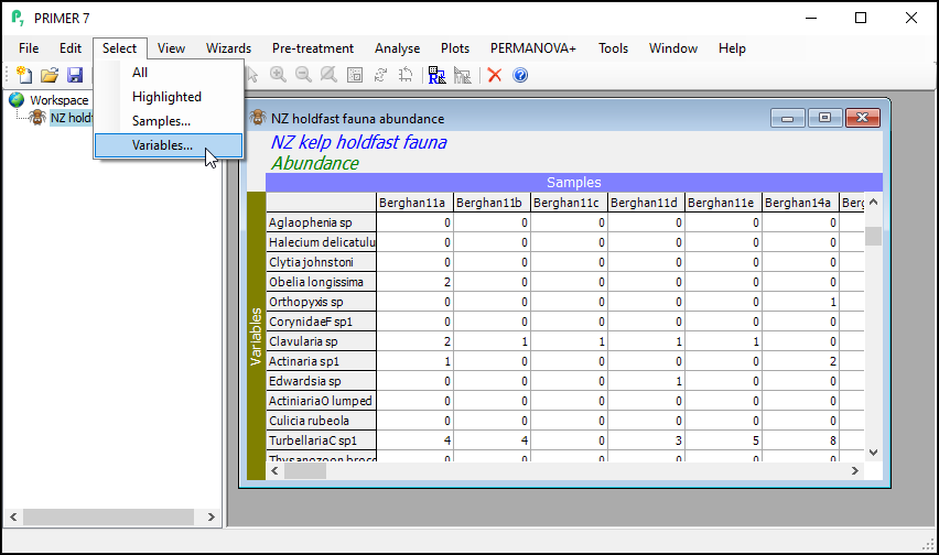
We wish to select just the mollusc species for the analysis.

1. From the 'NZ holdfast fauna abundance' data sheet, click Select > Variables...

2. In the 'Select Variables' dialog, choose ($\bullet$Indicator levels > Indicator name: Phylum) and click Levels....

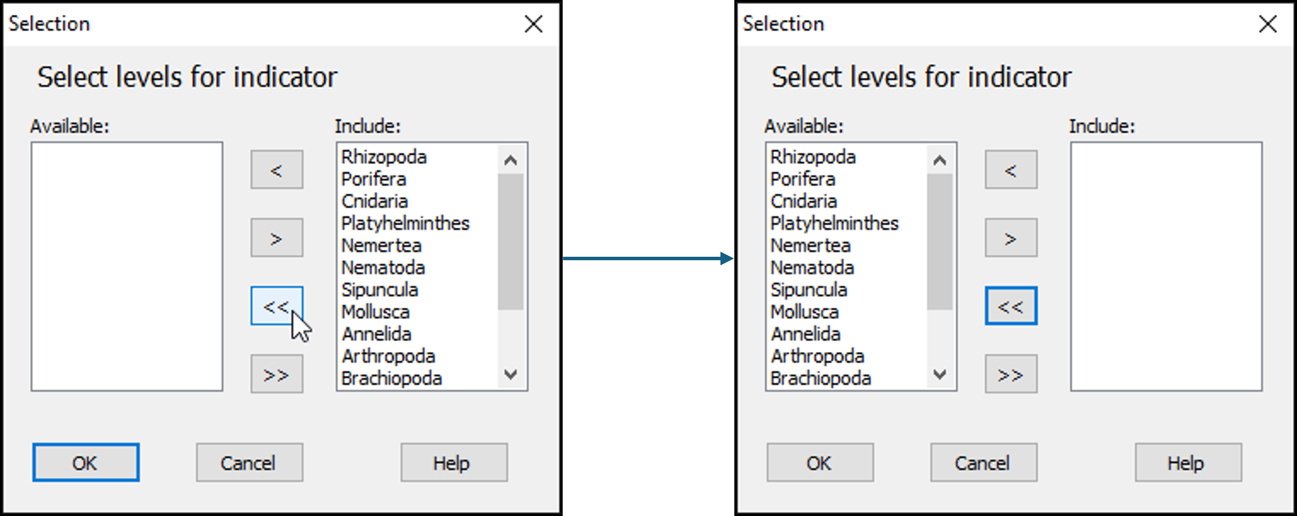
3. In the 'Selection' dialog, first move all of the phylum categories from the 'Include:' box (on the right) to the 'Available:' box (on the left) by clicking on the double-left-arrow button: .

4. Next, click on the word 'Mollusca' in the list of 'Available' phylum categories, and click on the single-right-arrow button:. This will move it to the 'Include:' box (right-hand side) of the 'Selection' dialog.

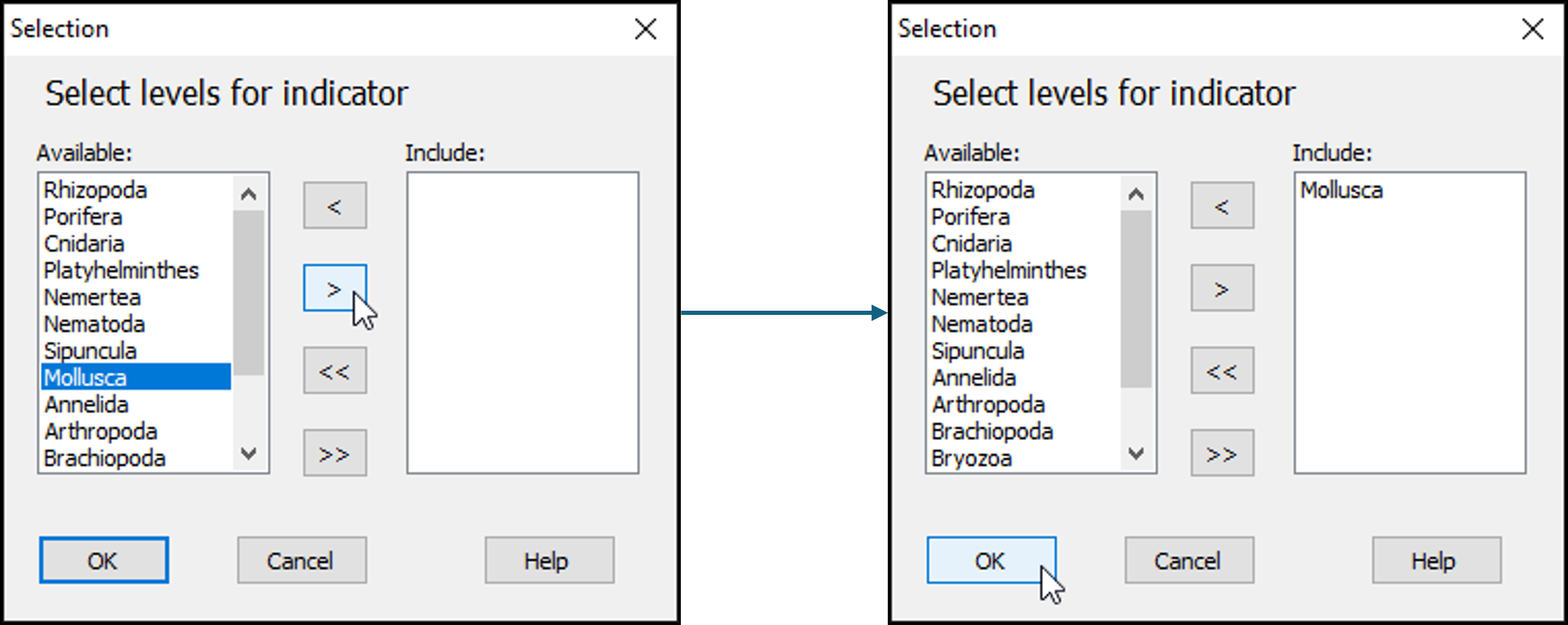
5. Click OK on the 'Selection' dialog, then click OK on the 'Select Variables' dialog.

Voila! Whenever you have selected a subset of data (this might be a subset of variables, as done here, or a subset of samples, or both), then the data matrix will have a turquoise background colour to indicate that you have done this, like so:

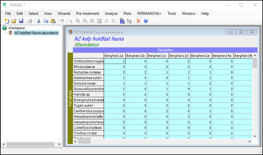
Any analyses done on a selected subset of data will only be performed on that subset. It is usually a good idea to duplicate and rename a selected subset of data, so as to keep any analysis done on that subset of data clear and separate from the (full) original dataset. Note that subsetting does not affect the original full data matrix of information in any way, which is still always there. You can clear any subset selection (of variables and/or samples) by clicking on Select > All to return to the full data matrix in its entirety. (The turquoise background colour will go away when you do that, and the formerly selected data will yet be highlighted in a purple-ish hue. Clicking on Select > Highlighted can then be used to re-instate the selection from before, if desired.)

Duplicate and rename a selected subset of data

From the subsetted data matrix, click Tools > Duplicate.

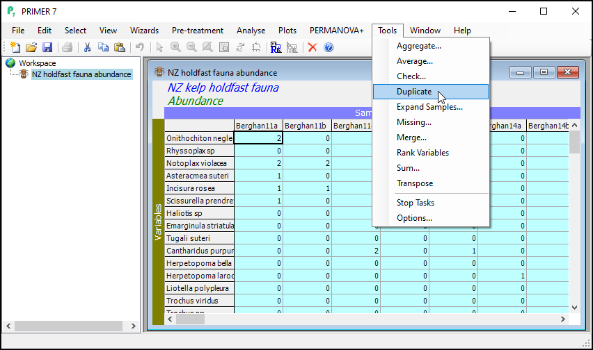
The result will be a new data sheet that contains only the subsetted data (in this case, only the molluscs). It shows up in the Explorer tree window. In the present example, this will (automatically) be called 'Data1'. It is no longer turquoise. The Duplicate routine was performed only on the subsetted (turquoise) data from the original sheet, yeilding this new data sheet, a subset of the original. If you click on Edit > Properties..., you will see that this new sheet now only has 105 variables ('Number of rows:').

Click, hover and click again on the name 'Data1' in the Explorer tree window (or click File > Rename Data or hit the 'F2' key) and type in a new name for the subsetted data sheet: Molluscs.

At this point, you might like to save your workspace. Click File > Save Workspace As... > (Filename: NZ_holdfast_molluscs.pwk).

Step 2: Jaccard resemblance

Calculate the Jaccard resemblance

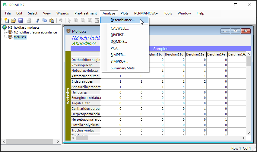
From the 'Molluscs' data sheet, click Analyse > Resemblance....

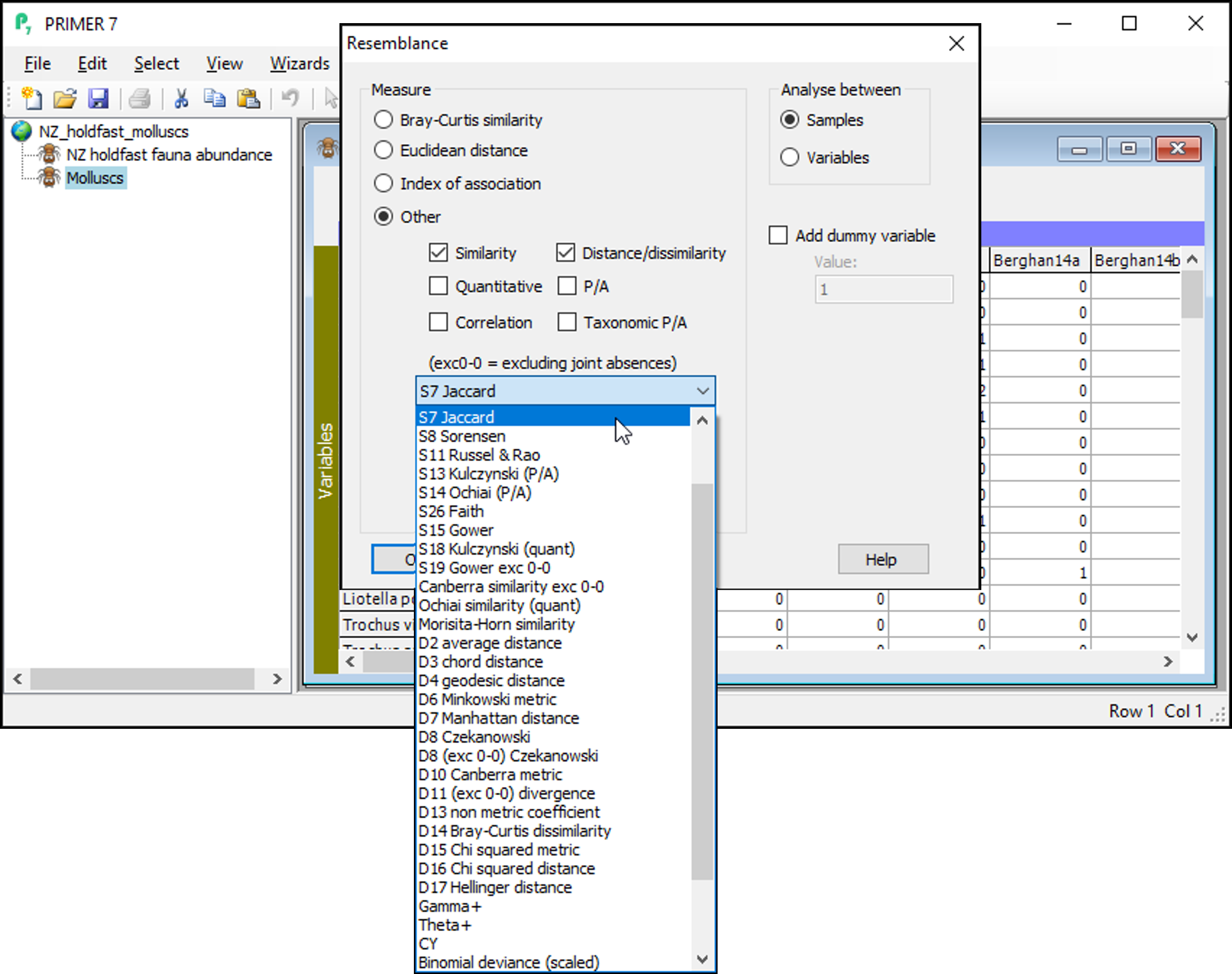
In the 'Resemblance' dialog, choose ($\bullet$Other) and then click on the drop-down menu to find 'S7 Jaccard', then click OK. (Note: 'S7' refers to the nomenclature used by Legendre & Legendre (2012) in their Chapter 7 on measures of ecological resemblance).

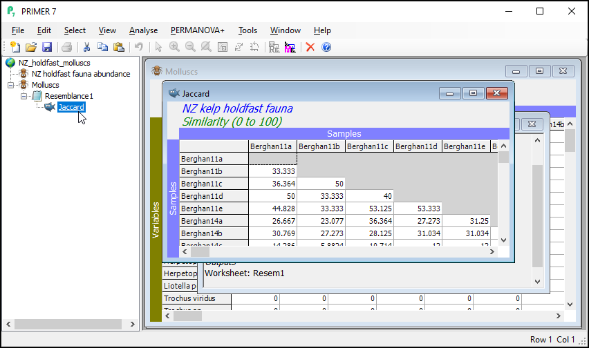
This produces a Jaccard similarity matrix among all pairs of holdfasts, called 'Resem1' by default. A nice feature of the Jaccard similarity measure is that it is directly interpretable as the percentage of shared species. For example, the first two holdfasts in the data matrix have a Jaccard similarity of 33.33%, so approximately one-third of the species that occur in either one or the other holdfast occur in both of them (i.e., are jointly present).

You can re-name this 'Jaccard' (click on the name 'Resem1' in the Explorer tree and hit the 'F2' key to re-name it), for clarity in what follows.

Step 3: Specify the design

PERMANOVA requires a design file to run.

You can see the Factors associated with the holdfast data matrix (or its resemblance matrix) by clicking on Edit > Factors.... These factors will be 'visible' to the PERMANOVA dialog that we will use to create our design file.

For this study, we want to create a design file that has all of the information that PERMANOVA will need to construct the correct partitioning, the correct pseudo-F ratios and the correct permutation algorithms to test every term in the model that is implied by the design. For this example, we have a fully hierarchical (nested) study design with three random factors: Locations, Sites (within Locations) and Areas (within Sites).

1. From the resemblance matrix ('Jaccard'), click PERMANOVA+ > Create PERMANOVA Design....

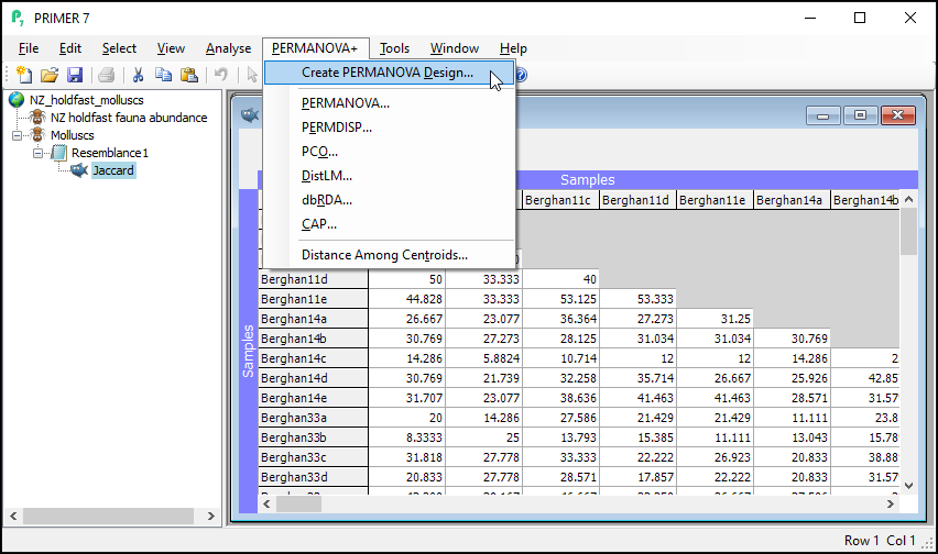
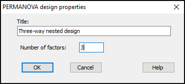
2. In the 'PERMANOVA design properties' dialog, pick a title for your design file, and indicate the number of factors. For the holdfast example, we will choose (Title: Three-way nested design)&(Number of factors: 3), then click OK.

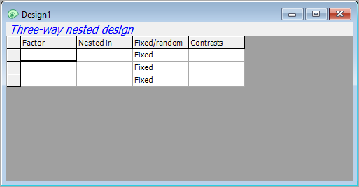
3. You will see an empty design file with three rows, one for each factor. Each row will correspond to a factor in your design. You will need to specify, in turn, the name and properties of each factor for the analysis in its own row.

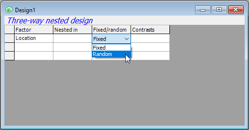
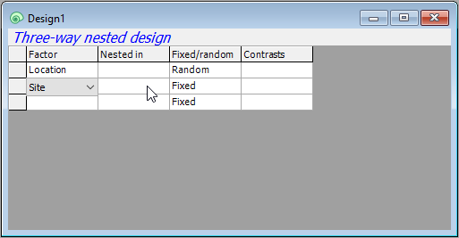
4. Location: First, in row 1, click in the blank cell under the word 'Factor', and you will see a drop-down menu listing all of the factors associated with the resemblance matrix from which this design file was created. Choose 'Location' to fill this cell. Location is not nested in anything, so we leave the second cell in row 1 blank. In the third cell of row 1, we have to specify that Location is a random factor, so click on the word 'Fixed' and change it to 'Random'.

4. Site: Next, we need to specify the second factor in the design in row 2 of the design file. Click on the cell in row 2 of the 'Factor' column (column 1) and choose 'Site'.

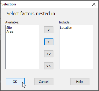
5. Sites are nested in Locations, so we have to specify that in column two ('Nested in') accordingly. Click on the cell in row 2 in column 2 and a 'Selection' dialog will pop up to allow you to choose the factors within which 'Site' is nested. You will need to click on the word 'Location' (in the 'Available:' box on the left), then on the single-right-arrow button () to move it over into the 'Include:' box (on the right), then click OK, like so:

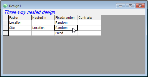
6. Make sure that the factor 'Site' is also specified in column 3 as 'Random'. (This happens automatically after specifying a nested term in column 2, because nested terms are, almost always, random factors.) Your design file should now look like this:

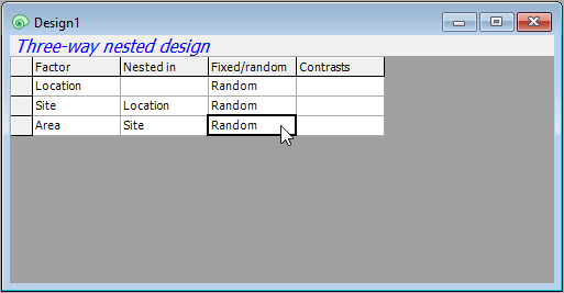
7. Area: Finally, we need to specify the third factor (Areas) correctly in row 3 of the design file. Under 'Factor' choose 'Area'. Under 'Nested in', specify 'Site', and make sure that column three has the word 'Random'. The final three-way nested design file should look like this:

Step 4: Run PERMANOVA

Once the design file is created, we are ready to go ahead with the PERMANOVA analysis.

1. Click on the 'Jaccard' resemblance matrix in the Explorer tree so that it is the active item in the workspace, then click PERMANOVA+ > PERMANOVA...

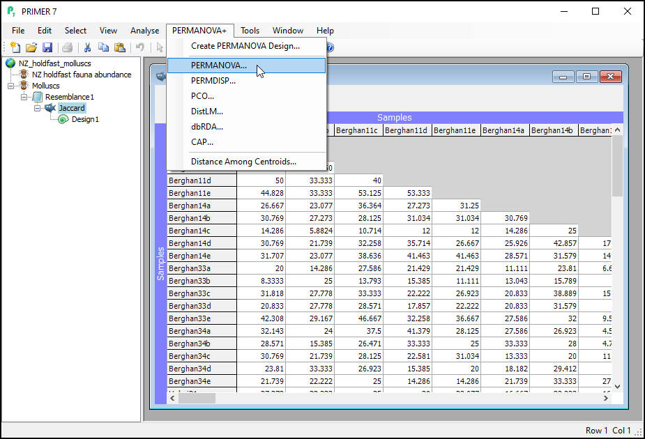
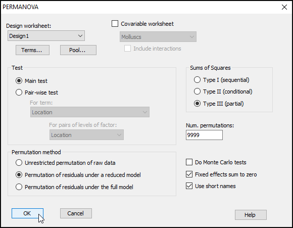
2. Check to see that the 'Design worksheet:' is Design1; this is the design file we created in the previous step that contains the three-way nested design. For the rest, we will keep most of the defaults in the PERMANOVA dialog, but it is wise to increase 'Num. permutations:' from 999 to 9999, as shown below, then click OK.

3. This produces an output file (called 'PERMANOVA1') in the Explorer tree. It shows:

• the details of the choices you made in the PERMANOVA dialog to run the analysis;
• the details of your experimental design; and
• the PERMANOVA table of results

as follows:

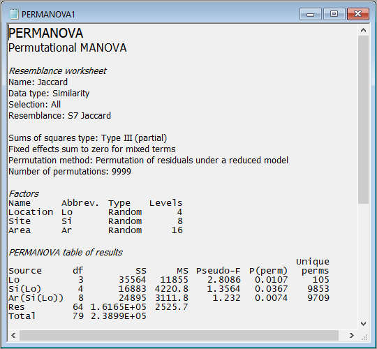
Interpretation

These results show that there is statistically significant variability in the identities of molluscs among holdfasts at each of the three spatial scales in the experimental design: Areas ($F_{8,64}$ = 1.23, $P$ < 0.01), Sites ($F_{4,8}$ = 1.36, $P$ < 0.05) and Locations ($F_{3,4}$ = 2.81, $P$ < 0.05). Note that the p-value for Locations is somewhat limited by the number of unique values of the pseudo-F statistic under permutation that are available here. Specifically, when we permute 2 samples per group (i.e., the 8 Sites) randomly across 4 groups (the Locations), there are just 105 unique values of pseudo-F that can be obtained, so the minimum possible p-value here is 1/105 = 0.0095).

Step 4 (continued): Key additional details about PERMANOVA in PRIMER

Following the PERMANOVA table of results, a suite of key additional details regarding the analysis can be seen in the PERMANOVA output file.

(Note: It is not necessary to fully unpack all of these details to continue on with the analysis and interpretation of results, but some information is provided here to highlight what makes the implementation of PERMANOVA in PRIMER so unique, surpassing all other software tools in its robust handling of multi-factorial experimental designs).

Additional details in the PERMANOVA output file include:

• details of the expected mean squares (EMS) for each term in the model;
• the construction of the pseudo-F ratios for each term in the model from the appropriate mean squares (along with the associated numerator and denominator degrees of freedom); and
• estimates of the components of variation for each term in the model in the space of the resemblance measure.

For example, scrolling down further in the output file from the PERMANOVA done on the holdfast data, we see:

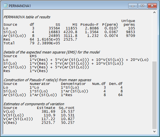
The implementation of PERMANOVA in PRIMER always uses expected mean squares (EMS) to construct correct tests for every term in the model; specifically:

• to construct the correct pseudo-F ratio; and
• to implement a permutation algorithm that
  • identifies the correct permutable units; and
  • accounts correctly for other terms in the model.

Of course, each term will require careful construction of its own test-statistic and its own permutation algorithm, both of which will depend on whether terms are fixed or random, whether there are other nested terms, covariates or interactions, etc. For unbalanced cases, the 'Type' of sum of squares is also important for the partitioning and correct construction of individual tests. All of these things can affect the EMS.

The EMS are also used to estimate the components of variation attributable to different sources of variation. These are not the same thing as raw $R^2$ values (as are typically used to compare the relative importance of individual predictor variables in regression models). In PERMANOVA, these are calculated in a directly analogous way to the unbiased univariate ANOVA estimators. The column labeled 'Estimate' expresses these components in squared dissimilarity units, and its square root ('Sq.root', interpretable as a sort of standard deviation in the space of the resemblance measure) is also provided.

In the present example, we can see that the greatest variation occurs at the smallest spatial scale - from holdfast to holdfast within a given area (i.e., the square root of 'V(Res)' is 50.257 in Jaccard % dissimilarity units). The sources of variation (in order of importance, as quantified by the PERMANOVA model) are: Residual > Location > Area > Site.

For more information about all of these key additional details provided in the PERMANOVA output file, please consult the PERMANOVA+ manual.

Step 5: Ordination of centroids

Having seen the results of a PERMANOVA analysis, it is natural to wish to see a visualisation of the patterns among centroids belonging to different groups or combinations of levels of different factors in the study design. In many cases, particularly if there is a large number of replicates in a complex study design, if one were simply to create an ordination of all individual sampling units, there would just be a lot of noise (the plot may look very messy), due to high residual variation. This tends to obscure salient patterns and important effects.

Ordination of sampling units (all replicates)

We can produce a non-metric MDS ordination of the holdfast data by starting from the Jaccard resemblance matrix and clicking on Analyse > MDS > Non-metric MDS..., taking all of the defaults, then clicking OK. The resulting configurations are very unsatisfactory with quite high stress, either in 2 dimensions (stress = 0.28, shown below), or 3 dimensions (stress = 0.20).

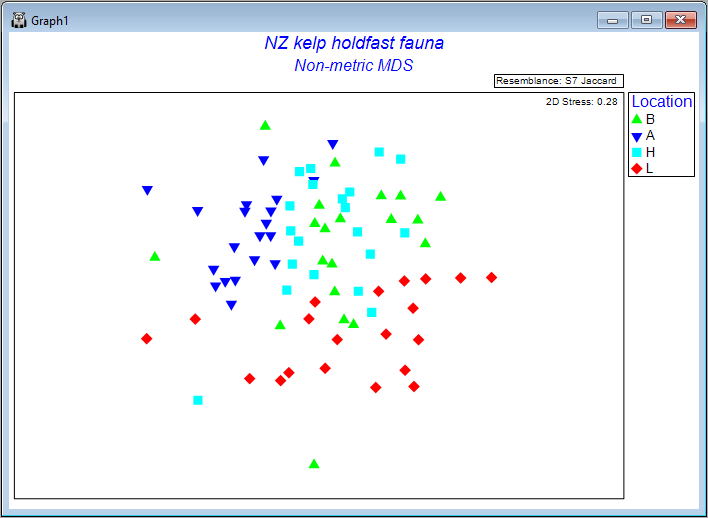
Seeing a bit of a 'mess' when we plot replicates like this is actually not too surprising in many cases, and particularly in this case, considering the very high variation (high turnover) in the identities of molluscs among holdfasts at small spatial scales (within areas), as seen on the previous page (recall that the residuals contributed by far the greatest source of variation to this system).

Ordination of distances among centroids

We can instead examine an ordination plot of the centroids in the space of the resemblance measure. In multi-factor designs when there is more than one factor and these factors are crossed with one another, we may need to created a single factor that consists of combinations of levels of the crossed factors (using Edit > Factors... > Combine...), but in the case of a fully nested design, and where nested factors all utilise unique labels (such as we have here), we can proceed without such a step.

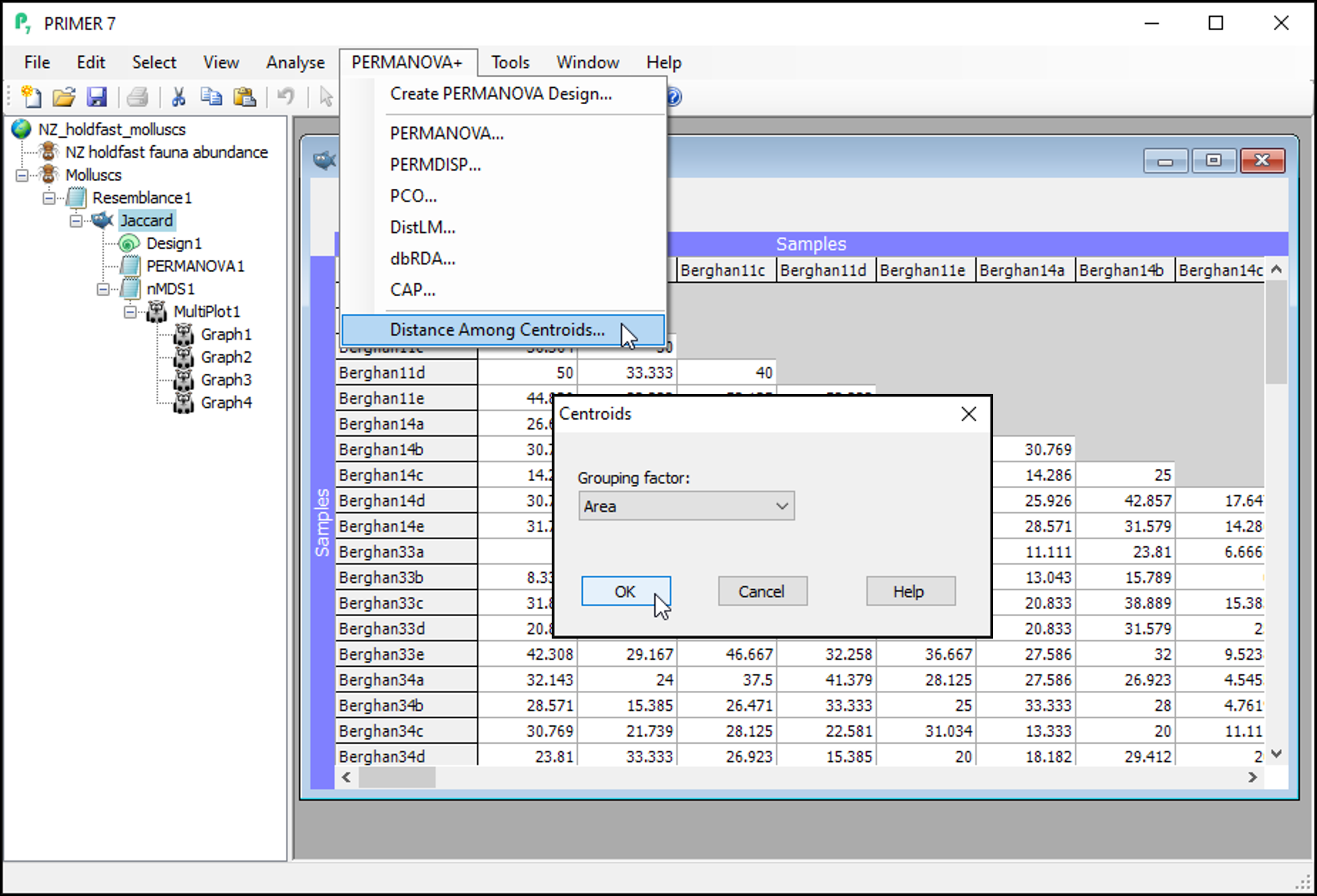
1. From the 'Jaccard' resemblance matrix, click PERMANOVA+ > Distances Among Centroids, then in the 'Centroids' dialog, choose (Grouping factor: Area), and click OK.

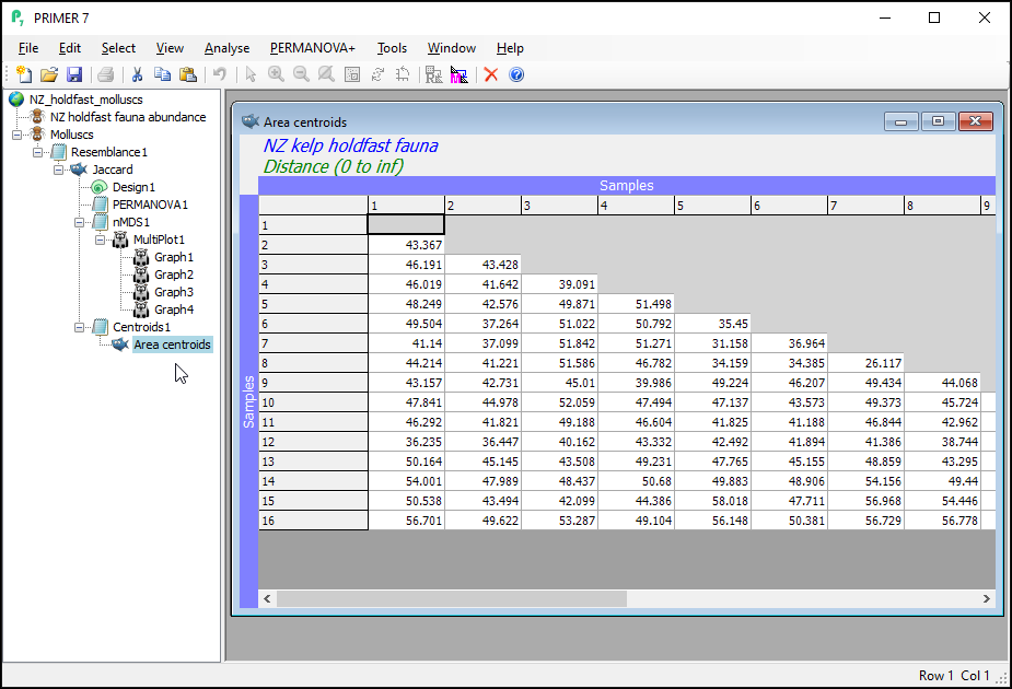
This will give you a matrix of Jaccard dissimilarities among the 16 Area centroids; each centroid being comprised of n = 5 replicate holdfasts within a given area. These are constructed in the space of the dissimilarity measure, which is not (quite) the same thing as calculating the arithmetic averages in the space of the original variables (i.e., that corresponds to a centroid in Euclidean space). In other words, these are the centroids just 'as PERMANOVA sees them' in Jaccard space, when doing the partitioning. You can re-name this matrix (from 'Resem1') to 'Area centroids'; i.e.,

2. From the 'Area centroids' resemblance matrix, click Analyse > MDS > Non-metric MDS..., take all the defaults and click OK.

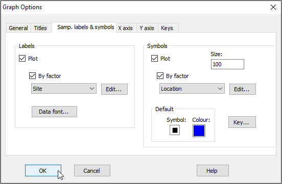
3. From the 2D nMDS (probably called 'Graph5'), click on Graph > Sample Labels & Symbols..., then choose (Labels > $\checkmark$Plot > $\checkmark$By factor > Site) & (Symbols > $\checkmark$Plot > $\checkmark$By factor > Location), then click OK.

The result is a much more interpretable ordination plot, with far lower stress, viz:

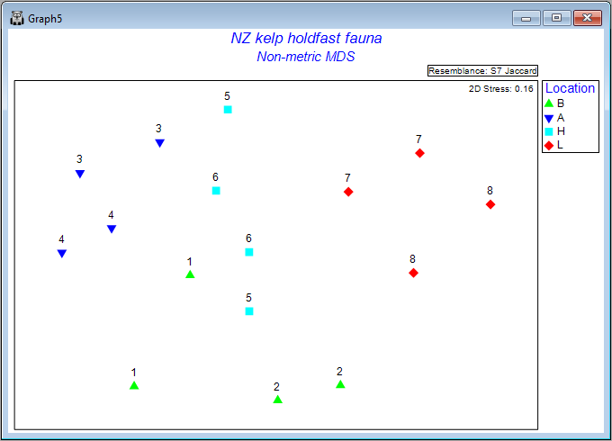
Each point now represents the centroid (in Jaccard space) for n = 5 holdfasts in a given area. The numbers identify the 8 different sites, and the colours correspond to the 4 different locations. The patterns we see here are consistent with what was learned from the PERMANOVA analysis. More specifically, we can see that, within any particular location, the variation from one area to the next (any 2 centroids having the same symbol and number) is fairly similar to the variation between the two sites (any 2 centroids having the same colour, but a different number), and also that variation among locations (different colours) exceeds this - all four locations are clearly distinguishable from one another on the plot.

Summary of the PERMANOVA analysis

A summary of the essential commands associated with performing this PERMANOVA analysis of the holdfast data according to the 3-factor hierarchical experimental design is given in the table below:

Step	To implement in PRIMER:
1. Select variable subset	From the original data sheet: click Select > Variables... > ($\bullet$Indicator levels > Indicator name: Phylum), click Levels...> (Selection > Include: Mollusca), click OK.
2. Jaccard resemblance	From the subset-selected data sheet: click Analyse > Resemblance > (Measure $\bullet$Other > S7 Jaccard) & (Analyse between $\bullet$Samples), click OK.
3. Specify the design	From the resemblance matrix: click PERMANOVA+ > Create PERMANOVA design... > (Title: Three-way nested design) & (Number of factors: 3), click OK. Fill in the appropriate details of the design in the design file.
4. Run PERMANOVA	From the resemblance matrix: click PERMANOVA+ > PERMANOVA... > (Design Worksheet: Design1) & (Num. permutations: 9999) & (default settings for the rest), click OK.
5. Ordination of centroids	From the resemblance matrix: click PERMANOVA+ > Distance Among Centroids... > Centroids > (Grouping factor: Area). From the resulting resemblance matrix among area centroids: click Analyse > MDS > Non-metric MDS..., take all the defaults and click OK. To specify labels and symbols: click Graph > Sample Labels & Symbols....