A Quick Guide to PRIMER
A quick guide to get you up and running with PRIMER software by Marti J. Anderson (2024)
- Citation
- 1. General information
- 2. Installing PRIMER software
- 3. Download manuals and examples
- 4. Getting data in to PRIMER
- 5. Example analysis pathway (CLUSTER, MDS, ANOSIM)
- An analysis of biotic data
- Step 1: Transformation
- Step 2: Resemblance
- Step 3: Cluster
- Step 4: Ordination
- Step 5: ANOSIM test
- Summary of the pathway
- 6. Some Wizards
- 7. Run a PERMANOVA
- Overview
- A three-factor hierarchical design
- Steps in a PERMANOVA analysis
- Step 1: Data selection
- Step 2: Jaccard resemblance
- Step 3: Specify the design
- Step 4: Run PERMANOVA
- Step 4 (continued): Key additional details about PERMANOVA in PRIMER
- Step 5: Ordination of centroids
- Summary of the PERMANOVA analysis
- 8. References
Citation
Anderson, M.J. (2024). "A Quick Guide to PRIMER." PRIMER-e Learning Hub. PRIMER-e, Auckland, New Zealand. https://learninghub.primer-e.com/books/a-quick-guide-to-primer.
1. General information
We're delighted that you've chosen to use PRIMER software. If you run in to any difficulties, we're here to help!
Getting in touch with us
For any up-to-date news, including details of upcoming courses, please consult our website: https://www.primer-e.com/.
Please report any bugs or technical problems to: tech@primer-e.com
For licensing and other general enquiries, contact the PRIMER-e administrative office at: primer@primer-e.com.
Resources
This guide is designed to get you quickly up and running with PRIMER software. More detailed information and examples of virtually all of the analyses offered by PRIMER and PERMANOVA+ software are found in the following manuals, all of which are downloadable from within the software, and are also available for perusal here on our Learning Hub:
- Clarke KR, Gorley RN, Somerfield PJ & Warwick RM. (2014). Change in Marine Communities, 3rd edition. PRIMER-E Ltd: Plymouth, UK.
- Clarke KR & Gorley RN. (2015). PRIMER v7: User Manual / Tutorial. PRIMER-E Ltd: Plymouth, UK.
- Anderson MJ, Gorley RN & Clarke KR. (2008). PERMANOVA+ for PRIMER: Guide to Software and Statistical Methods. PRIMER-E Ltd: Plymouth, UK.
System requirements
For PRIMER version 7 and PERMANOVA+:
- Operating system: Windows 10 or 11 (must be Windows XP or later).
- CPU: Modern Intel or AMD processor
- RAM: 8 GB or more
- Hard-disk space: 100 MB or more
Note that PRIMER will not run natively on Apple Mac OSX, but can be run via virtualization software or BootCamp. Also, to be able to read and write Excel worksheets, you will need Excel 2000, or later, installed.
PRIMER software is a device-independent installation; it is not for terminal servers.
2. Installing PRIMER software
Overview
Here we provide instructions for the download and installation of PRIMER 7 (with PERMANOVA+). Please read this information in conjunction with our End-User Licence Agreement (EULA).
These instructions are applicable to enable activation of single end-user licences of the software for any of the following sectors:
- COMMERCIAL (Private enterprise, consultant, for-profit organisation)
- PUBLIC (Government/State agency, museum, not-for-profit organisation)
- ACADEMIC (University/College faculty, technicians and postdoctoral researchers)
- STUDENT (Full-time student at undergraduate, Masters or PhD levels)
Your purchased Licence Key (32 characters) will authenticate the software. Your licence is identified by a unique serial number, which you should use in any communication with us regarding your licence.
Trial mode vs Fully-featured version
PRIMER 7 (with PERMANOVA+) software can be downloaded and installed either in trial mode, (free for 30 days) or as a full version, which requires payment for a licence activation key.
In trial mode, all PRIMER 7 and PERMANOVA+ routines are available, but you will be unable to save or print, and all graphics you produce will be watermarked, so presentation-standard output is unobtainable from screen grabs. You will be able to access a small sub-set of example data files from within the “Help” menu (although not the full, more extensive set of example data files). The trial version has a 30+ day expiry date, with an additional grace period, but will then cease to operate – reinstallation of the trial version on the same machine is not possible.
The full version is activated by entering your Licence Key in the Install routine. A valid installation key can be purchased at any time from PRIMER-e and inputting that to the Install routine when on-line will remove all such printing and saving restrictions and watermarks. Once purchased, your single end-user License Key can be used to activate the fully-featured PRIMER software on up to two (2) computers (e.g., at home and at work). You will then be able to save, print and produce graphics without a watermark and access the full set of extensive example data files.
If you need to move your PRIMER software to a new machine (or re-image the machine), first uninstall your Licence Key. If you are unable to uninstall the Licence Key (e.g., due to machine failure), contact us on tech@primer-e.com, and our technical team can reset your Licence Key for installation onto a new machine.
PRIMER 7 and the PERMANOVA+ add-on
The trial software includes both PRIMER and PERMANOVA+, but if only the base package of PRIMER is purchased (without the PERMANOVA+ add-on), then the PERMANOVA+ routines will not be enabled and those menu items will no longer appear. If you purchase PRIMER 7 with PERMANOVA+, your Licence Key will enable all routines.
If a single-user PERMANOVA+ licence, for use with PRIMER 6, is already registered to you then no further purchase of PERMANOVA+ is needed when you upgrade to PRIMER 7 – it operates in essentially the same way with PRIMER 7 as it did with PRIMER 6. When you upgrade, you will be given a single installation key, and your PRIMER 7 software will include the PERMANOVA+ add-on as well, due to your pre-existing licence for this.
How do I know if I have the PERMANOVA+ add-on?
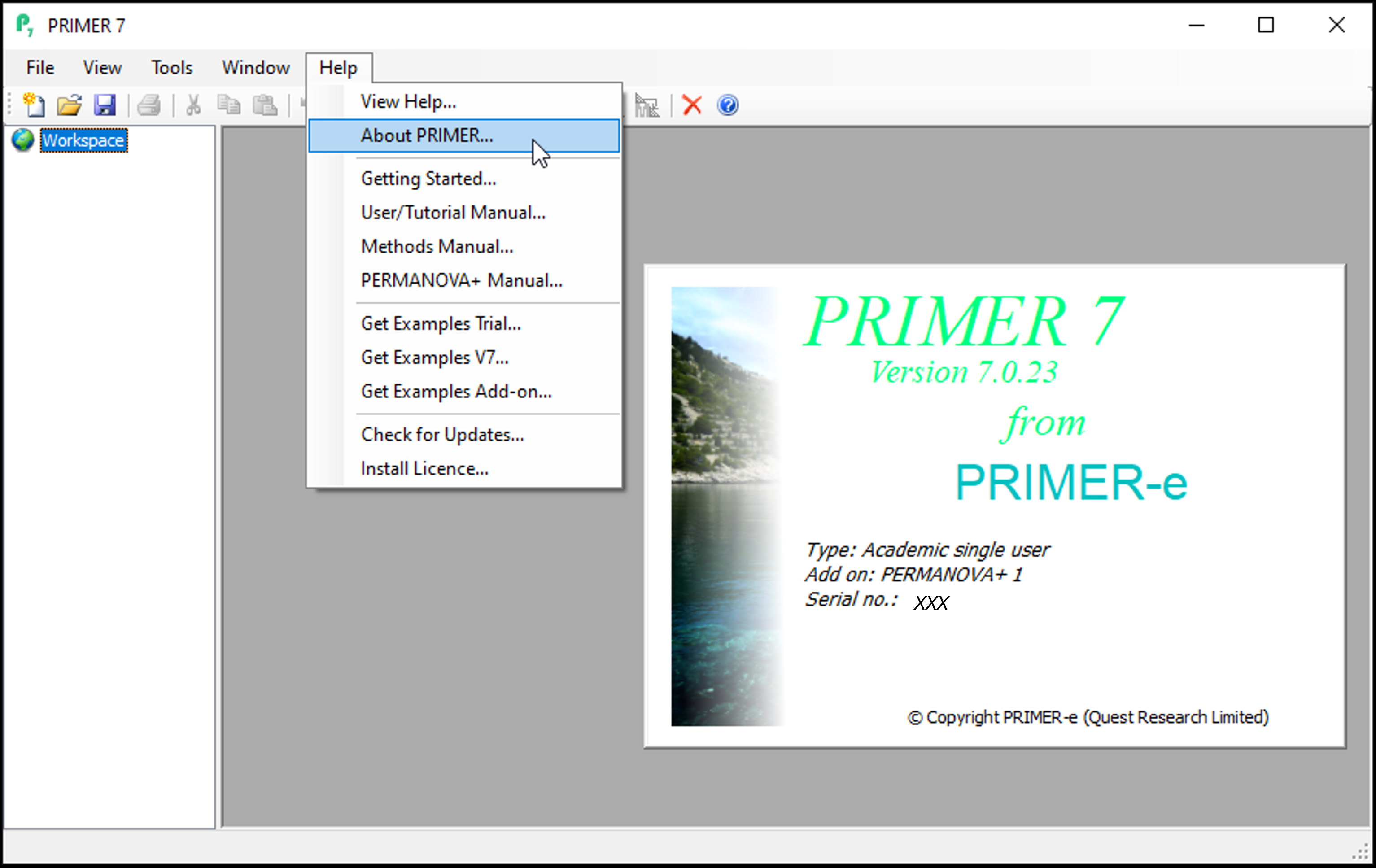
Once PRIMER is installed, click on Help > About PRIMER.... The splash screen will show the add-on as being present if you have purchased it (as in the image below). If your licence key includes PERMANOVA+, then you will also see the PERMANOVA+ menu item appear within PRIMER when you select a resemblance matrix in the workspace tree; almost all the routines in PERMANOVA+ begin from a chosen resemblance matrix.
Check for updates
Click on Help > Check for Updates.... If an update is available (as in the image below), click on Update and follow the instructions.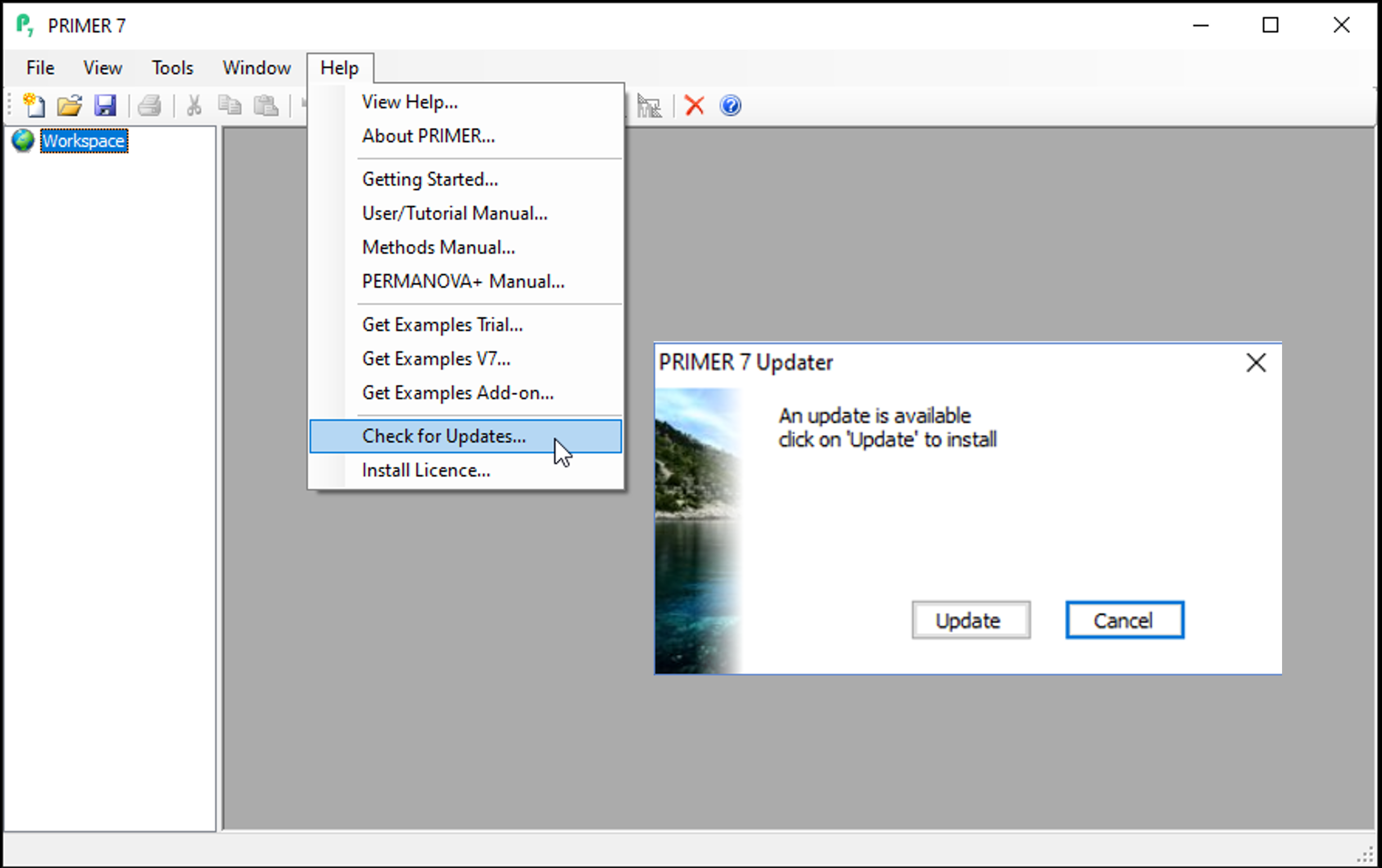
Download the installer
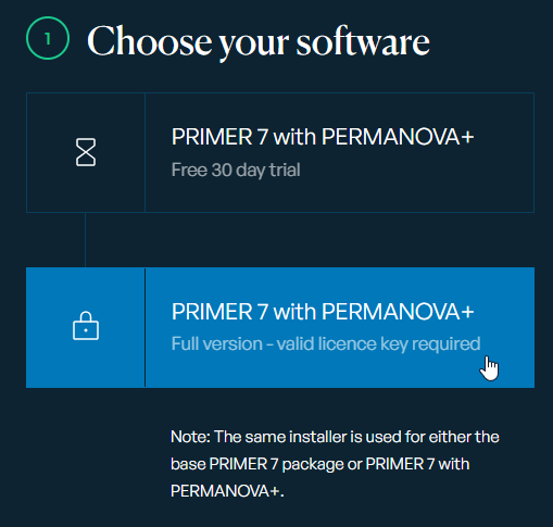
- First, head to our download page. Where it says 'Choose your Software', choose 'PRIMER 7 with PERMANOVA+, Full version - valid licence key required'.
- Enter your details and tick the box $\checkmark$'I'm not a robot' (you will need to successfully follow the ensuing verification instructions associated with this statement), then click on the green button to 'Download software'.

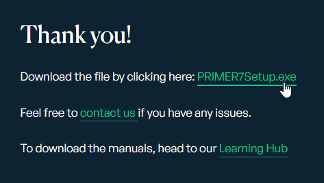
- On the screen that says 'Thank you!', click on the link to download the executable file for installation: "PRIMER7Setup.exe". This file will then be available for you in the 'Downloads' folder on your machine.
Install the software
Once the download has completed, double click on the downloaded installation file ('PRIMER7Setup.exe') to start the installation process.
Install and activate PRIMER
Install the software
Important note: You will require administrator permissions on your user account to install PRIMER on your computer. If you do not have these permissions, please contact your IT team who should be able to assist you in installing PRIMER.
- Double click on the downloaded installation file ('PRIMER7Setup.exe') to start the installation process:
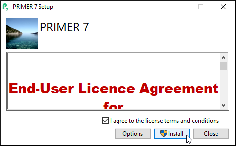
- A 'PRIMER 7 Setup' window will appear. Please read the 'End-User License Agreement for PRIMER'. If you agree to the terms and conditions of this EULA, click on the tick-box $\checkmark$'I agree to the license terms and conditions' and then click on Install.
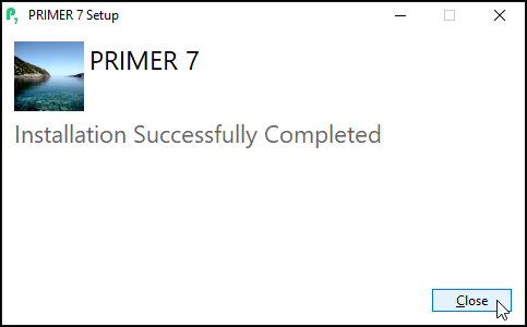
- Follow the prompts and once the installation has successfully completed, click Close.
Activate the licence key
You must be connected to the internet to carry out the licence authentication, though after that the software can be run when not connected.
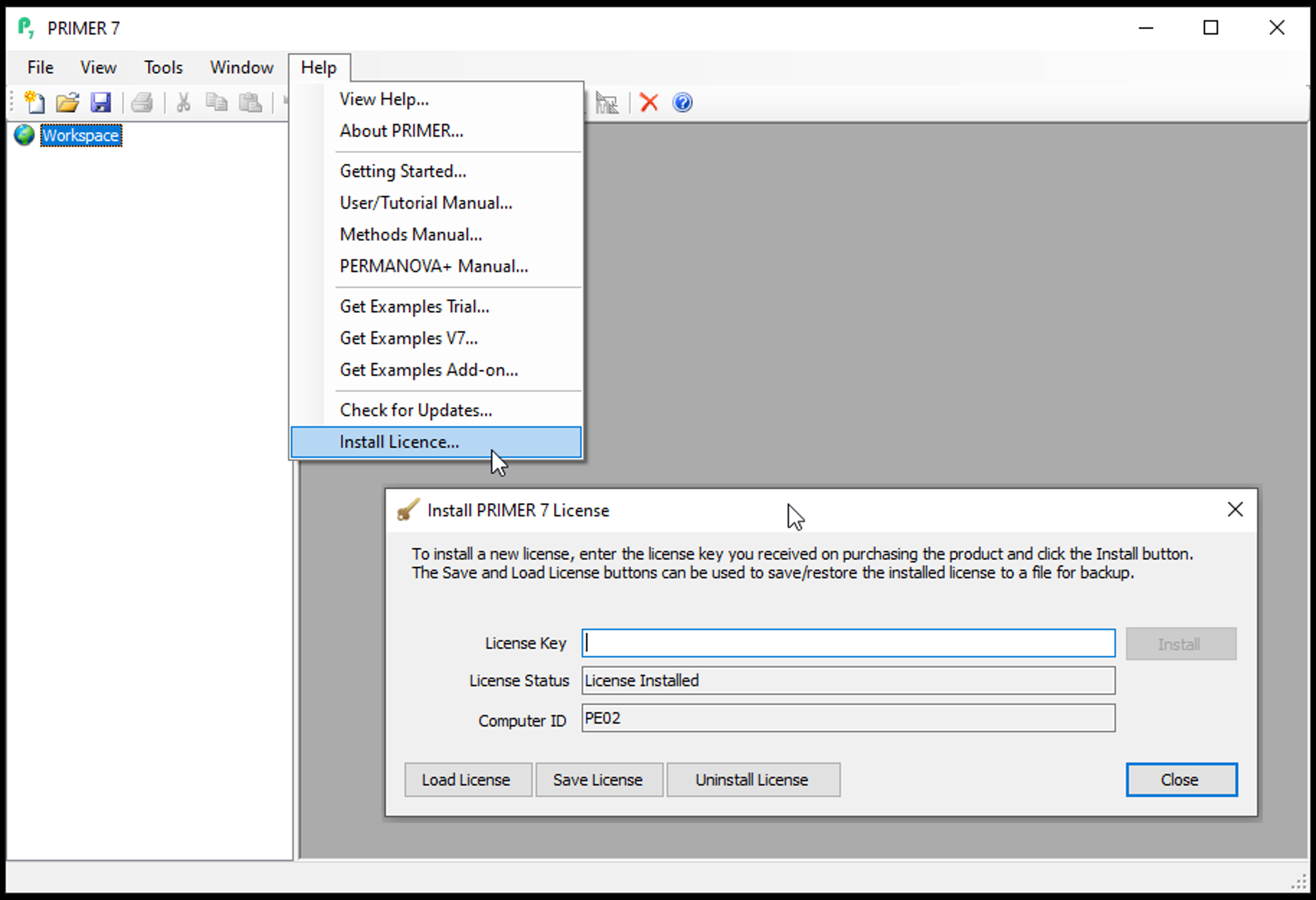
- Double-click on the desktop icon to launch the PRIMER 7 software.
![]()
-
Click on the Install License button in the 'Welcome to PRIMER 7' dialogue box. (Note: If you have already exhausted your 30-day trial, a message may appear to advise you that 'Your evaluation period has expired'. If that happens, simply click on Install License to carry on with the instructions to activate your licence.)
-
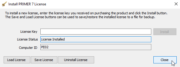
Copy and paste your 32-character Licence Key code into the 'License Key' box and click on Install. (Note: the installation key shown in the image below is not a valid licence key - you have to paste in your own!)
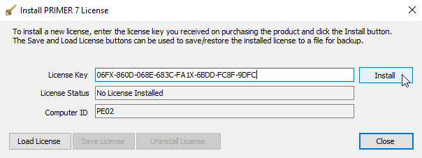
- In the 'License Status' box it will tell you it is 'Authenticating', then it will indicate 'License Installed'. Click on Close.
The installer will then automatically open your PRIMER-e software.
Note: If your firewall denies access to our authentication server and your IT service cannot unblock this, please contact the PRIMER-e office for assistance to authenticate your licence: primer@primer-e.com.
Uninstall / re-install PRIMER
If you need to move the PRIMER software to a new machine (or re-image the machine), first uninstall your Licence Key (when connected to the internet) and then uninstall the PRIMER software, if required. Uninstall-reinstall cycles are intended to cope with the purchase of new machines (not regular movements between a larger body of PCs). A given Licence Key will permit 4 such uninstall-reinstall cycles only.
Important note: You will require administrator permissions on your user account to uninstall PRIMER from your computer. If you do not have these permissions, please contact your IT team who should be able to assist you in uninstalling PRIMER.
To uninstall your Licence Key:
- Open PRIMER and click on Help > Install License....
- In the 'Install PRIMER 7 License' window, click on Uninstall License.
- In the 'Confirm License Uninstall' window, click on Yes to confirm. It will 'De-authenticate' before telling you there is 'No License Installed'. Click on Close.
To uninstall the PRIMER software from your machine:
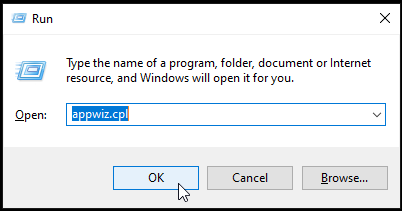
- Press the 'Windows Key' and the 'R' key on your keyboard at the same time to open the 'Run' window.
![]() + R
+ R
- In the 'Run' window, type 'appwiz.cpl', then Click OK .
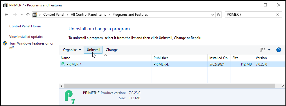
- A new window will pop up with a list of installed programs on your computer. Look for 'PRIMER 7' in the list (programs are shown alphabetically), or type 'PRIMER 7' in the 'Search Programs and Features' box (located in the top right-hand corner of the dialog), and then select the PRIMER 7 program shown in the list with your mouse so that it is highlighted.
-
With the PRIMER 7 software highlighted, click the Uninstall button at the top of the list, then just follow the prompts to finish uninstalling the PRIMER software. Please note, you must have administrator permissions on your user account to perform this operation.
-
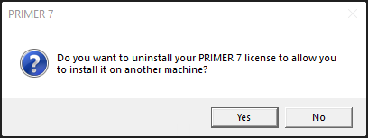
If you have a valid PRIMER license activated when uninstalling PRIMER software from your machine, you should receive a prompt that says "Do you want to uninstall your PRIMER 7 license to allow you to install it on another machine?" You should click "Yes". The only exception is if you are planning on reinstalling PRIMER on the same machine again, then click "No" and follow the procedure to "Install and activate PRIMER".
(Note: When you next attempt to start up PRIMER 7, it may tell you that 'Your evaluation period has expired'. You will be able to re-install the Licence anew by clicking on Install License and entering your current or a new Licence Key.)
To uninstall your current Licence Key and reinstall with a new Licence Key
- Open PRIMER, select Help > Install License.
- In the 'Install PRIMER 7 License' window, click on Uninstall License.
- In the 'Confirm License Uninstall' window, click on Yes to confirm this action. It will 'De-authenticate' before telling you there is 'No License Installed'.
- Next, copy and paste the new Licence Key into the 'License Key' box and click on Install.
Reset a Licence Key
If you are unable to uninstall the software from your machine before installing on a new machine (e.g., machine failure), please email us directly at primer@primer-e.com with your name, licence serial number (or Licence Key) and a request to reset your licence. We’ll check the information you provide against our records and let you know once the licence key has been re-set and ready for re-installation (within 1-2 business days). If you are not the registered end-user, please note that we will need the registered end-user to get in touch with us to confirm your request.
'The number of installations has been exceeded'
When installing the software on a new machine, you may see an error message that says, 'The number of installations allowed for this licence key has been exceeded'. If you have multiple machines with PRIMER installed, simply uninstall PRIMER from one of them to allow you to install it on a different machine. If you are unable to do this, please email us directly at primer@primer-e.com with your name, licence serial number (or Licence Key) and a request to re-set your licence.
3. Download manuals and examples
(from within the PRIMER software)
Download manuals
The following manuals can be downloaded from within the software itself:
- Getting Started...: Clarke, K.R., Gorley, R.N. (2015) Getting started with PRIMER v7. PRIMER-e: Auckland, New Zealand.
- User/Tutorial Manual...: Clarke KR, Gorley RN (2015) PRIMER v7: User Manual/ Tutorial. PRIMER-e: Auckland, New Zealand.
- Methods Manual...: Clarke KR, Gorley RN, Somerfield PJ, Warwick RM (2014) Change in marine communities: an approach to statistical analysis and interpretation, 3rd edition. PRIMER-e: Auckland, New Zealand.
- PERMANOVA+ Manual...: Anderson MJ, Gorley RN, Clarke KR (2008) PERMANOVA+ for PRIMER: Guide to software and statistical methods. PRIMER-e: Auckland, New Zealand.
You must be connected to the internet to download the manuals. Simply click on the Help menu item in PRIMER, then choose which manual you wish to download as a pdf. Each of these manuals are a substantial tome and together these will provide you with virtually all the information you will need to run the routines, analyse your data, produce graphics and interpret relevant output.
Once downloaded the manuals can then be read and searched (at any time, whether you are connected to the internet or not) and can be printed, if you wish, for your own personal use. The manuals are also freely available for perusal on our website's Learning Hub.
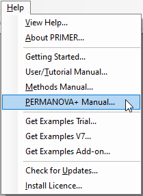
Please note that the PERMANOVA+ Manual will only be available from within the software if you have purchased the PERMANOVA+ add-on (see 'How do I know if I have the PERMANOVA+ add-on?').
Download example data
You must be connected to the internet to download the example datasets.
- Examples Trial...: available when the software is in free-trial mode;
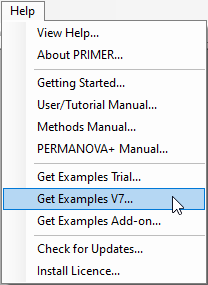
- Examples V7...: to accompany the base PRIMER package; and
- Examples add-on...: to accompany the PERMANOVA+ add-on package.
You can download and save these to a folder of your choice when prompted. These datasets provide a wealth of examples from the literature, and they are referred to extensively throughout the manuals.
We highly recommend working slowly through the manuals and replicating the examples given there with the example datasets provided as an excellent way to familiarize yourself with the program and its many routines. Example datasets are also used extensively in our international workshops. For details of upcoming workshops across the globe, consult our website: https://www.primer-e.com.
4. Getting data in to PRIMER
Opening example data
Data from the Fal estuary
Example datasets in PRIMER can be obtained via the Help menu item. In trial mode, click Help > Get Examples Trial..., and you can download the following four files of example data (held in a folder called 'Examples Trial') to a location of your choice:
- Fal environment.pri (measured values for 12 environmental variables x 27 sites)
- Fal environment.xls (same as above, but in Excel format)
- Fal nematode abundance.pri (abundances of 62 nematode species x 27 sites)
- Fal nematode taxonomy.agg (taxonomic hierarchy for the 62 nematode species)
These data come from a study of benthic infaunal communities in soft sediments from 27 sites over five creeks of the Fal estuary, SW England ( Somerfield et al. (1994a) , Somerfield et al. (1994b) ). Sediments at these sites were contaminated to varying degrees by heavy metals, from historic mining activities. Both faunal counts (nematodes) and environmental measures were obtained from the same set of sites. (Note: the extension *.pri indicates a file containing a data matrix that has been saved in PRIMER 7's own internal (binary) format, unreadable by other software or earlier versions of PRIMER. Similarly, the *.agg extension indicates an aggregation-type file for PRIMER.)
Open the Fal data in PRIMER
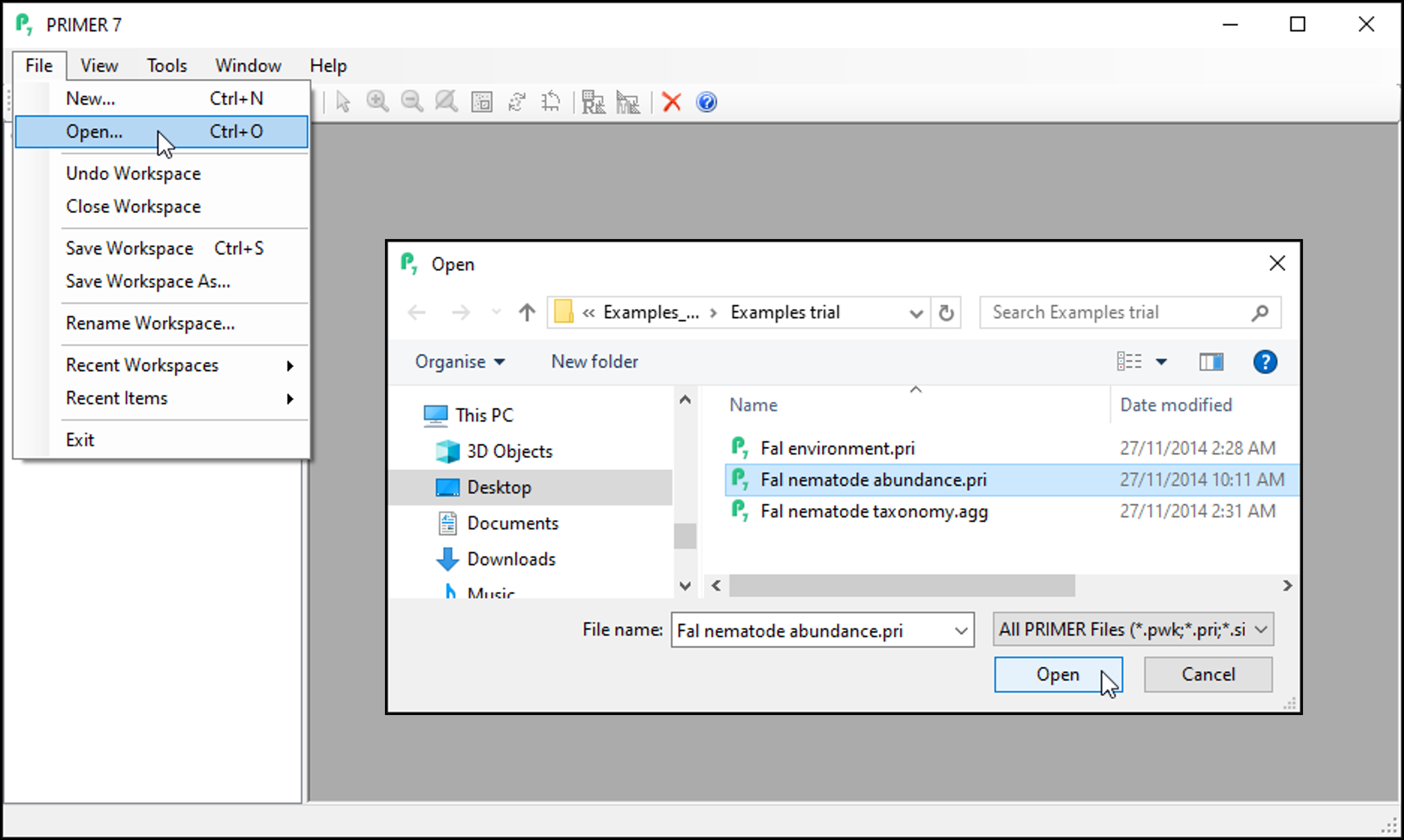
To open the species-by-samples data matrix, launch PRIMER, then click File > Open from the main menu, navigate to the 'Examples trial' directory in the location you have specified, and select 'Fal nematode abundance.pri'. Click Open to display the species matrix.
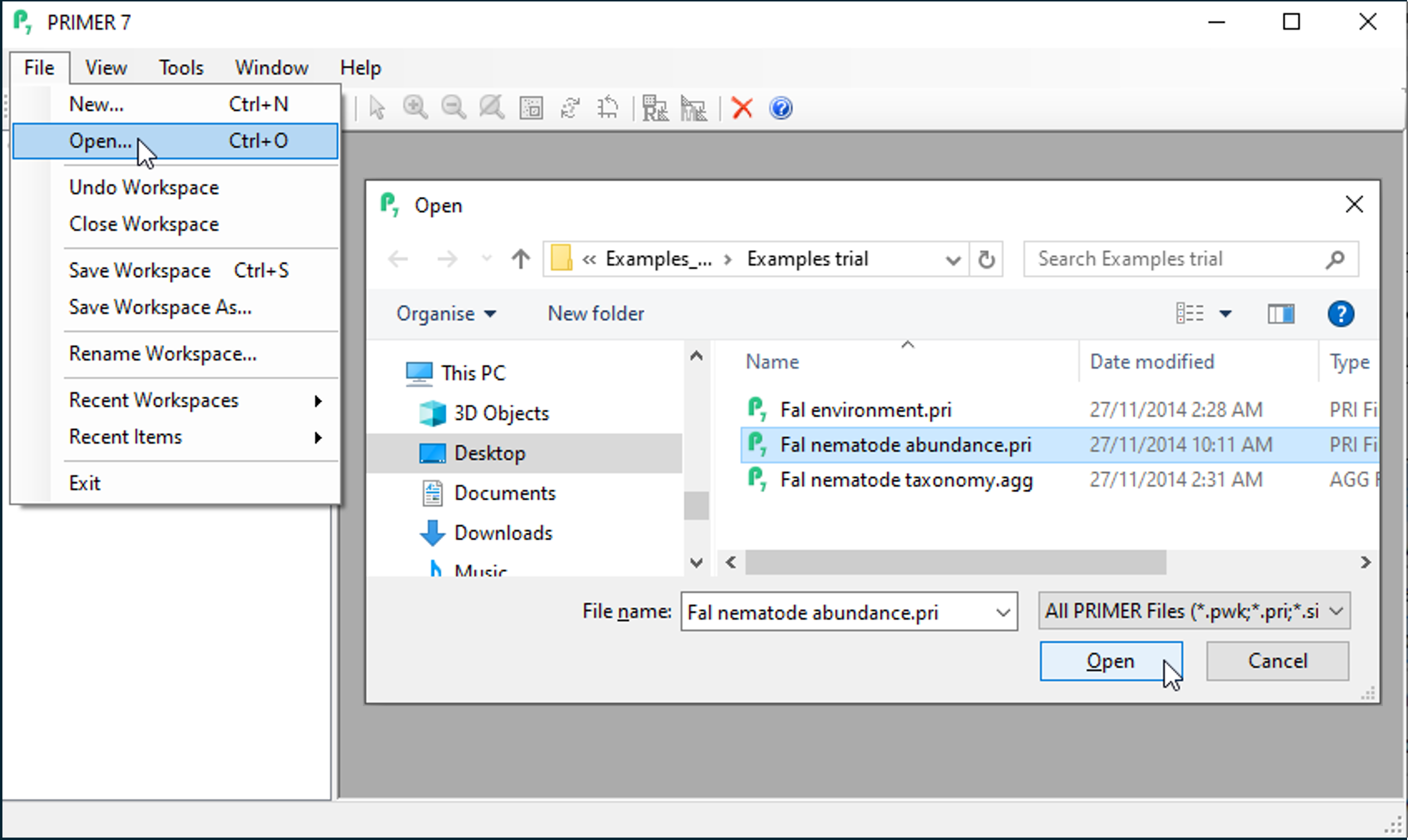
Alternatively, because this is a PRIMER file type (*.pri), you can instead use Windows Explorer to navigate to your specified folder and just double-click on the file name. This will launch a PRIMER session, with the data matrix open in the PRIMER desktop.
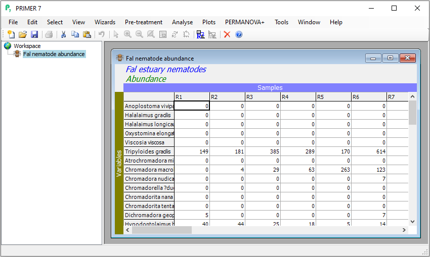
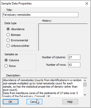
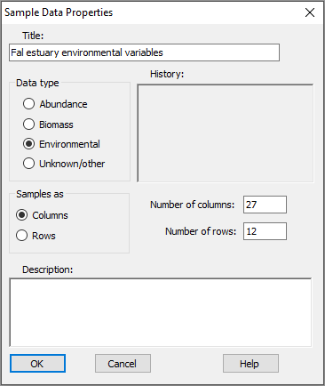
Properties of the data
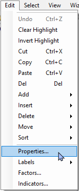
Click on Edit > Properties and you will see that PRIMER-format *.pri sheets carry other information about the data matrix as well, including:
- Title,
- Data type,
- Array size (number of columns and rows),
- Orientation (whether samples are found in columns or rows),
- a Description, and
- a History of what pre-treatments (such as a transformation) have been applied to them.
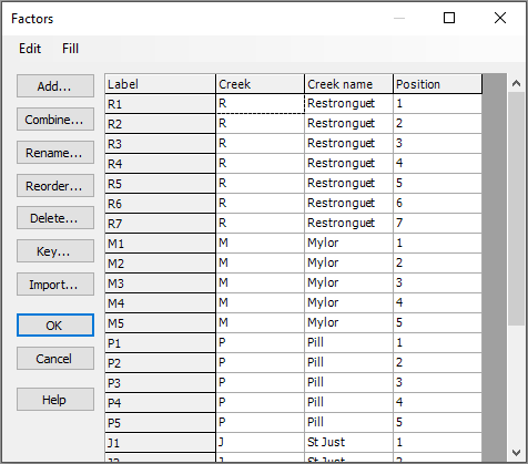
Factors associated with the data
Click on Edit > Factors, and you can see that a subsidiary sheet of three factors is also linked to this worksheet: 'Creek', a single-letter abbreviation for the creeks, the full 'Creek name' and a numeric 'Position' factor identifying the location of each sampling site down each creek.
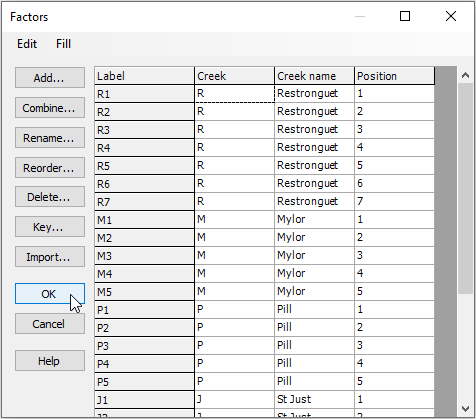
Note that additional factors could be added here by clicking Add, and also combinations of levels of existing factors can be created by clicking on Combine.
Importing data from Excel
Step 1. Ensure your data are in a format suitable for import into PRIMER
Suppose we have a dataset in Excel that is already in a suitable format for import into PRIMER. The environmental data from the Fal estuary provides an example of this. These data are found in the file 'Fal environment.xls' and consist of values for each of 12 environmental variables measured from sediments collected from 27 sites across 5 tidal creeks in the Fal Estuary (available from within PRIMER by clicking Help > Get Examples Trial..., as seen in the last section).
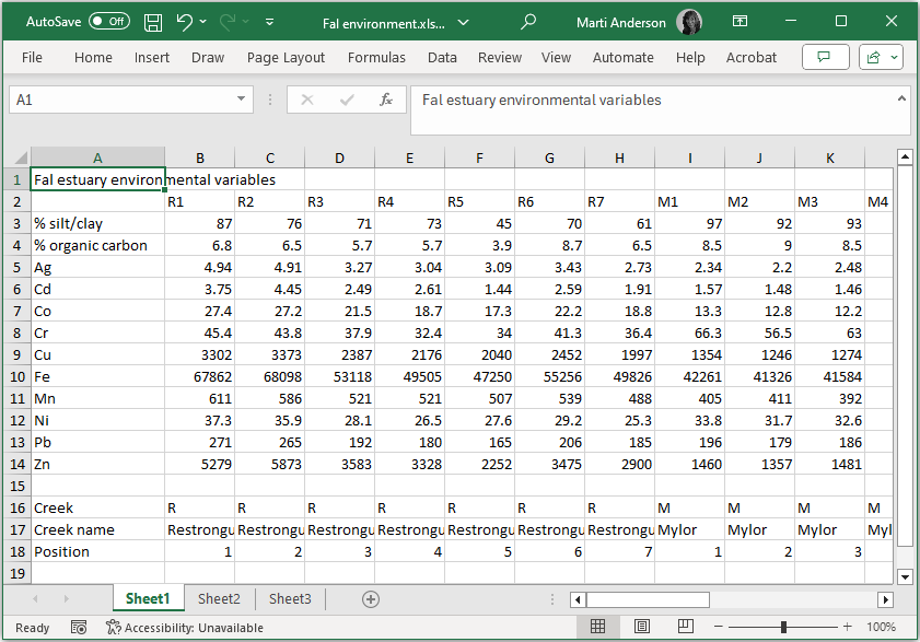
Important things to note about this file:
- There is a title for the dataset ('Fal estuary environmental variables') in the very first (upper left-hand) cell (A1). This title is optional, but handy as a naming convention.
- The cell immediately under the title (cell A2) is empty.
- There are column labels ('R1', 'R2', ...) in row 2. These are unique labels for the sampling units (Sites in this case).
- There are row labels ('%silt/clay', '% organic carbon', ...) in column A. These are unique names associated with each variable.
- The entries for every cell in the matrix of data itself (beginning with cell B3) all contain numerical values only. There are no non-numeric characters. This means that you may not use 'NaN' or 'NAN' to denote missing values. If data are missing from a cell, then it should be left blank. In addition, symbols such as '<' or '>' (for 'less than' or 'greater than') are similarly not permitted or accepted as valid data values within the data matrix.
- In this example, the variables are rows and the sampling units (sites) are columns. It is perfectly ok to have this formatted the other way around, with variables as columns and sampling units as rows. You will specify the orientation of your data matrix explicitly when you import your Excel file into PRIMER.
This format must be adhered to precisely, with no extra blank rows or columns, or extra headers, otherwise PRIMER will not be able to open it successfully.
Other things to note:
- Factors: You can label the sampling units as belonging to a level of one (or more) factors by skipping a line at the bottom of the matrix and placing this 'factor information' there. In the above image you can see that there are three factors: 'Creek' (row 16), 'Creek name' (row 17) and 'Position' (row 18).
- Indicators: You can similarly label variables as belonging to particular groups in the same manner; this is done along the other margin of the data matrix (e.g., after skipping a column, for this example). This might be useful for doing analyses on subsets of variables belonging to different types, such as physical vs chemical variables. In a case where variables are species, one might want to consider subsets of variables corresponding to families, functional groups, etc.
Inclusion of one (or more) factors (to specify groups of samples) or indicators (to specify groups of variables) is optional. If you have more than one factor, then these are given one after the next (in adjacent rows); do not put blank rows between multiple factors. The initial single blank row (or column) is there simply to demarcate the difference between the data matrix itself and additional information about the data matrix upon import.
Step 2. Open PRIMER and import the data from Excel
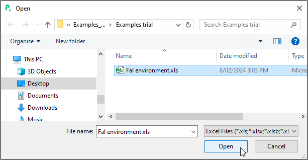
Once your Excel file is ready, open up PRIMER and choose File > Open. Look at the bottom of the dialog box and you will see next to the words 'File name:' that the only files that PRIMER can see is: 'All PRIMER Files...'. Click on 'All PRIMER Files...' and change this to 'Excel Files...'. Once you have done this, you should be able to browse and see the Excel data file that you want.
- Click on the name of your Excel file in the browser (here it is 'Fal environment.xls'), then click Open.
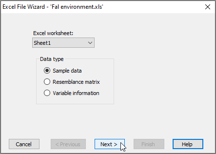
- This will initiate PRIMER's Excel File data-import Wizard. Choose the name of the specific sheet within your Excel file that contains your data and the type of data you are importing. Here, we have (Excel worksheet: Sheet1) & (Data type $\bullet$Sample data), then click Next >.
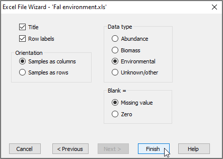
- Choose the correct orientation, type of data and the meaning of blank entries (if any). For this example, we have (Orientation $\bullet$Samples are columns) & (Data type $\bullet$Environmental) & (Blank = $\bullet$Missing value), then click Finish.
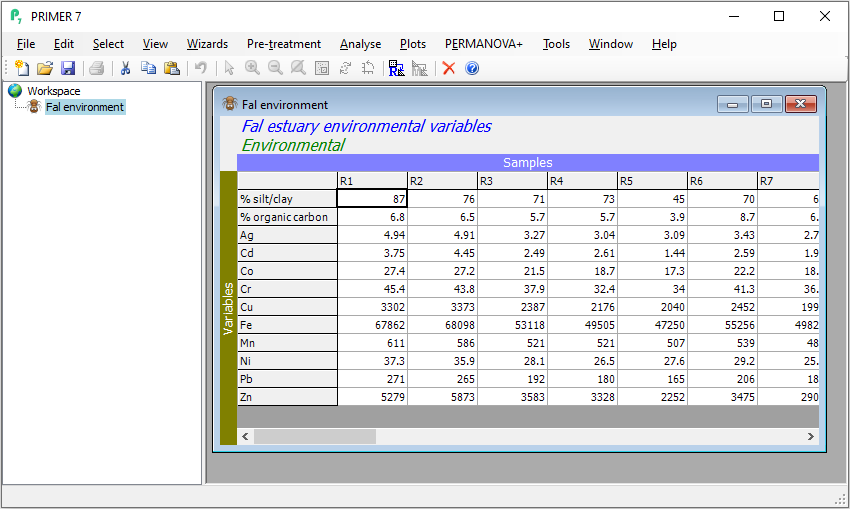
- You will now see your data file has been imported and is nicely displayed in the PRIMER workspace. It appears in its own window, and its name also appears in the 'Explorer tree'-type window shown on the left-hand side of the PRIMER desktop.
Now that the data are in PRIMER, it is a good idea to do some post-import data checks.
Post-import data checks
Check the orientation
After import, make sure you have specified the orientation correctly by examining the labels on the columns and rows of the data frame. For example, after importing the Fal environmental data from Excel (see the previous page), you can see that the columns are 'Samples' (a periwinkle-coloured strip across the top) and rows are 'Variables' (an olive green-coloured strip along the left margin).
If you happen to get this the wrong way around (e.g., if your variables are actually columns instead of rows), this can easily be changed (swapped around) by choosing Edit > Properties and toggling the radio button for 'Samples as' to either '$\bullet$Columns' or '$\bullet$Rows', whichever is appropriate.
Check the properties, factors and indicators
To be sure that the import has been fully successful, including all data points, factors and indicators that may have been included in your original Excel file, you can see additional information attached to your data matrix by clicking on your imported dataset in PRIMER, and doing the following:
- Look at the data properties, size of the matrix, etc.: Click Edit > Properties.... Note that you can add a useful 'Description' of your data into this dialog if you like. (For the Fal environmental dataset, we can see there are 12 variables and 27 sites, etc.).
- Look at the Factors (if any): Click Edit > Factors.... (For the Fal environmental dataset, you will see the same three factors of 'Creek', 'Creek name' and 'Position' that we saw in the Excel file).
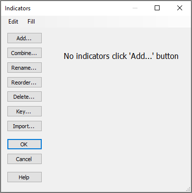
- Look at the Indicators (if any): Click Edit > Indicators.... (For the Fal environmental dataset, there were no indicators, but you could add some here, if you wish).
Run PRIMER's data-checking tool
As an additional option, you can run PRIMER's internal data-checking tool to find and identify certain other features that might be present in your data, including:
- Missing values,
- Negative values,
- Duplicate samples,
- Duplicate variables,
- All-zero samples,
- All-zero variables, and/or
- Estimated values
To run this routine, start by clicking on your datasheet, then click on Tools > Check...:
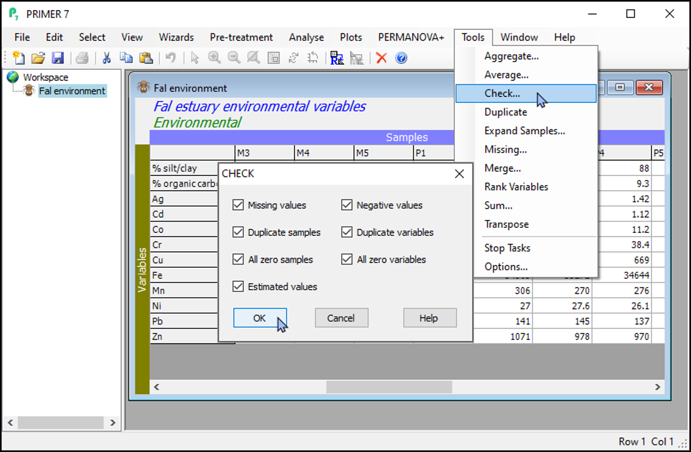
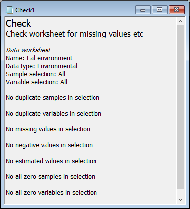
For the Fal environmental data, none of these features occurred (see below), and we are ready to proceed with subsequent analyses.
Save your data & workspace
Save your data in PRIMER (*.pri) format
To save a data sheet in PRIMER (*.pri) format, click on the data sheet inside the PRIMER workspace you want to save and click File > Save Data As....
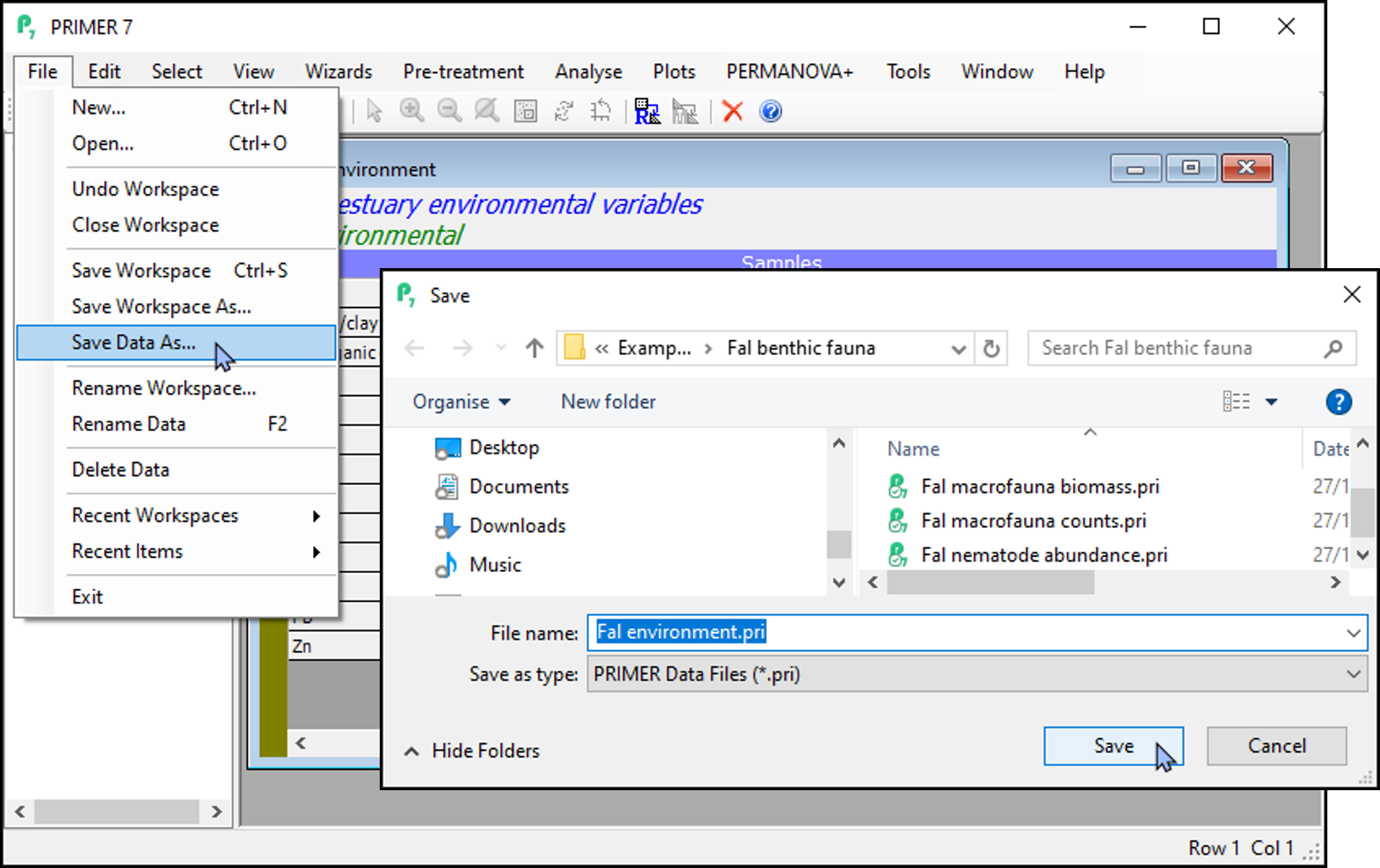
Note the default file-type for saving a data file is 'PRIMER Data Files (*.pri)', as shown in the box labeled 'Save as type:' in the 'Save' dialog. You can change this (by clicking in the 'Save as type:' box) in order to save the data in some other format of choice, such as *.txt, *.csv *.xls, *.xlsx, or in a PRIMER format compatible with older versions of the PRIMER software.
Save your entire PRIMER workspace (*.pwk)
Generally, you will want to save your data plus all of the work you have done in PRIMER to analyse that dataset. To save the entire PRIMER workspace, click File > Save Workspace As...
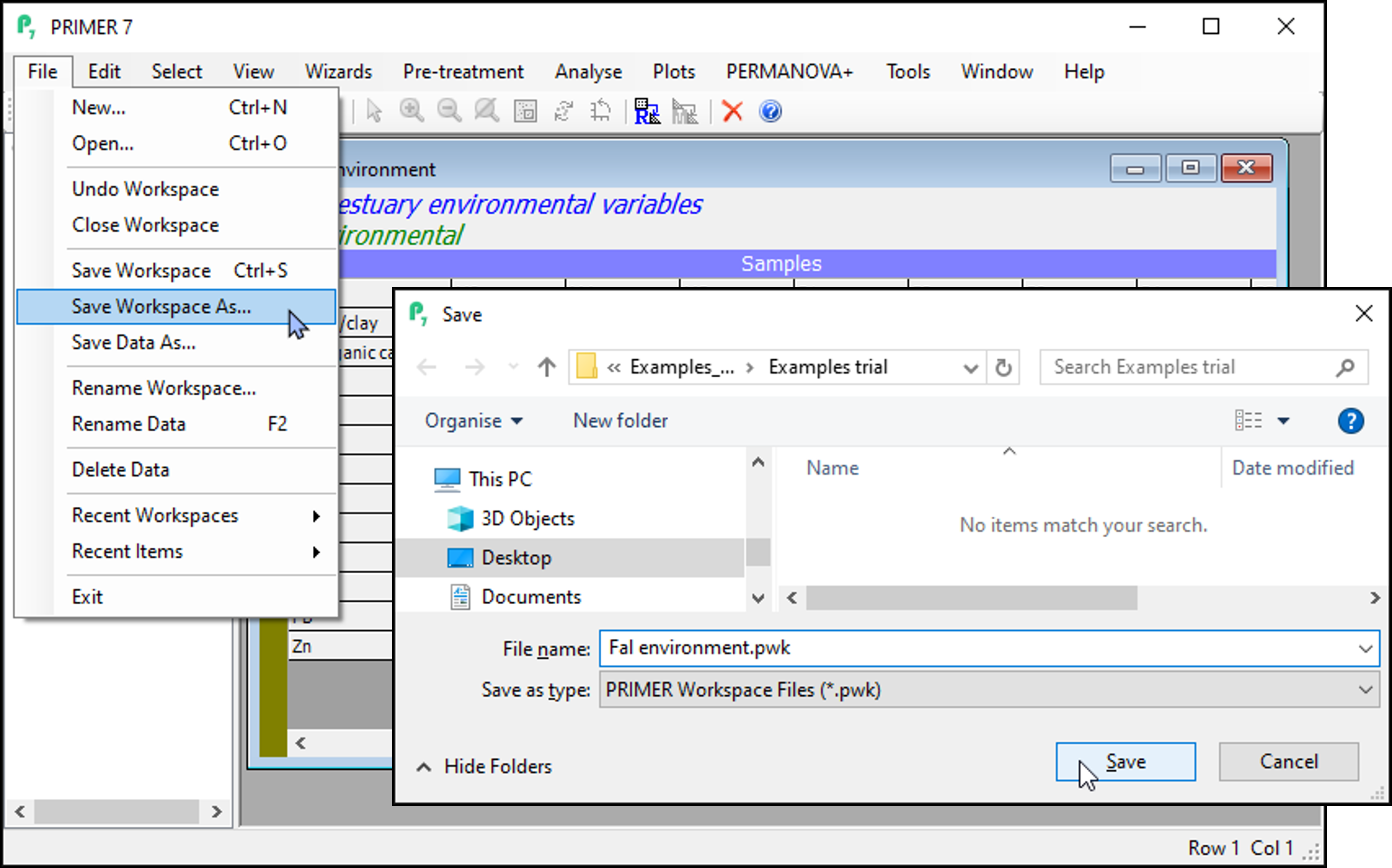
Type the file name you wish (e.g., Fal environment.pwk), and click Save. This will save the entire PRIMER workspace (not just the datasheet), including all elements you may have created during the PRIMER session (e.g., data, graphics, analyses, etc.), all of which you are able to navigate and see listed (in hierarchical fashion) within the Explorer tree window on the left-hand side of the open PRIMER workspace.
A PRIMER workspace file is identifiable by using the file extension *.pwk in the file name. Double-clicking on a file with this extension will open up that entire PRIMER workspace within the PRIMER software.
5. Example analysis pathway (CLUSTER, MDS, ANOSIM)
An analysis of biotic data
Rationale
Multivariate data are very complex and can be difficult to analyse and interpret. Each variable can be considered its own dimension, with its own story to tell. Thus, when there are a lot of variables (e.g., if we have sampled occurrence, abundance, or biomass of individual species in a community, and each species is a variable), then we have a very high-dimensional system to consider. We can choose to analyse each variable individually, but this would be time-consuming if we have a lot of variables. Also, for biotic data, many species are rare, so our data will be riddled with a large number of zeros - it would be difficult to characterise anything about individual rare species on their own. Furthermore, what we are usually aiming to do is to characterise and analyse the whole community simultaneously and how it may be changing through time or space, or in response to some experimental treatments (such as human impacts or management scenarios, etc.).
When analysing multivariate biotic data (especially those having a large number of variables), a useful approach is to base the analysis on a resemblance measure (i.e., a dissimilarity or similarity measure), calculated among the sampling units (e.g., Clarke (1993) , Anderson (2001a) , McArdle & Anderson (2001) ). A resemblance measure such as Bray-Curtis captures the ecological idea of turnover in the identities and relative abundances of species beween any pair of sampling units ( Clarke et al. (2006) , Anderson et al. (2011) ). For many routines in PRIMER, the fundamental starting point is a resemblance matrix, which expresses (numerically) the (dis)similarities between every pair of samples.
Before calculating a resemblance matrix, some pre-treatment of the data (sometimes in more than one way) is usually desirable. For assemblage data, an overall transformation can be used to reduce the dominant contribution of abundant species towards Bray-Curtis similarities. For example, a fourth-root transformation will down-weight the influence of highly-abundant taxa.
From a resemblance matrix, we may readily apply the following methods (Fig. 5.1):
- Cluster analysis, to help characterise inter-sample relationships, showing potential groups of similar samples;
- Ordination, to help visualise inter-sample relationships in a small number of dimensions (usually 2 or 3); and
- Hypothesis-testing, to formally test a particular null hypothesis of interest, such as H0: 'There are no differences in community structure among different (a priori) groups of samples'.
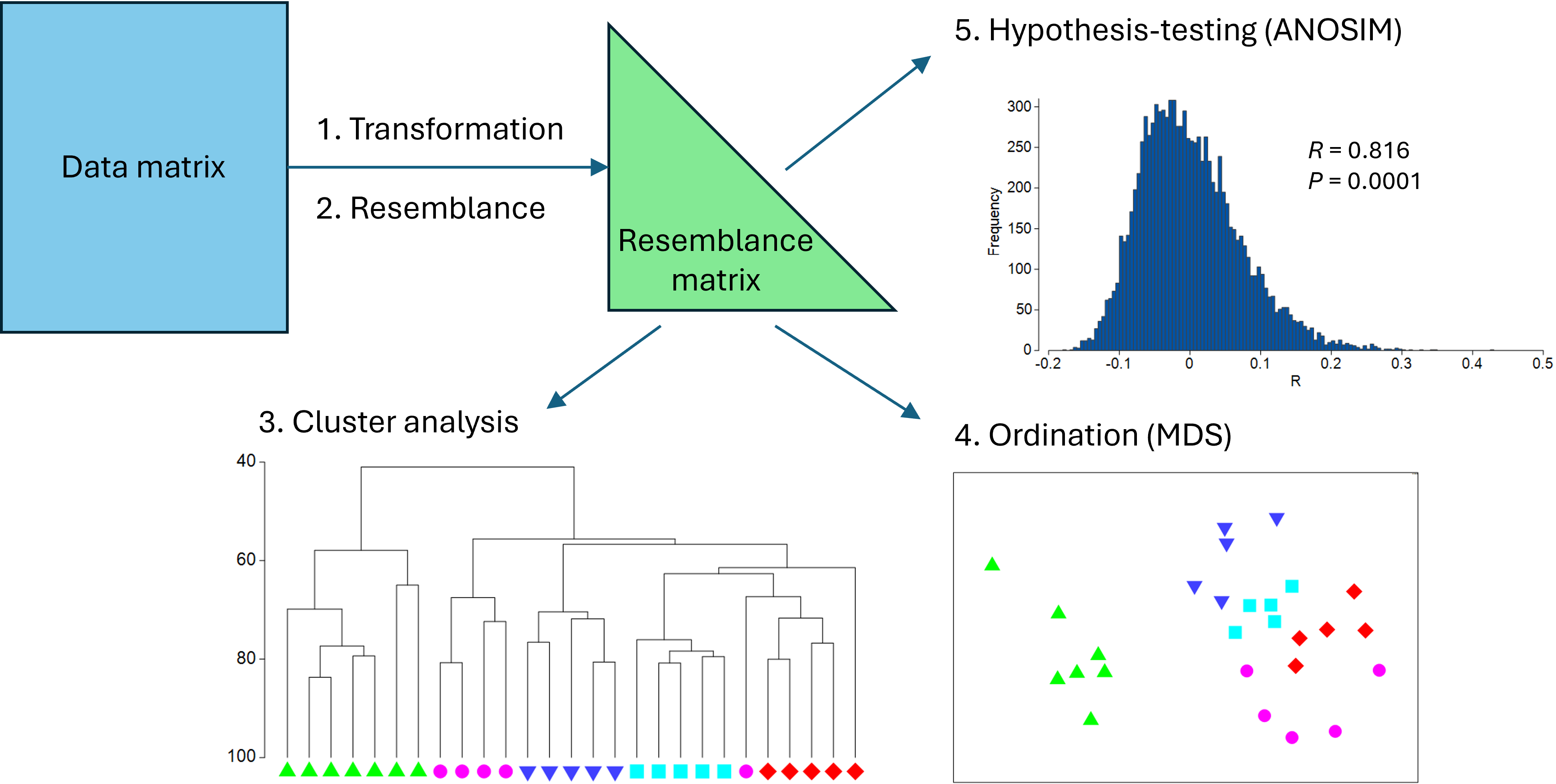
Fig. 5.1. Schematic diagram of a simple multivariate analysis pathway, including transformation, resemblance, clustering, ordination and hypothesis-testing.
Some steps for analysis
In what follows, we shall take the 'Fal nematode.pri' example dataset in PRIMER and proceed along a simple multivariate analysis pathway according to the following steps:
- Apply a fourth-root transformation to the data (all variables).
- Calculate the Bray-Curtis resemblance among all pairs of samples.
- Calculate a hierarchical group-average cluster analysis of the samples to produce a dendrogram.
- Create a non-metric multi-dimensional scaling (nMDS) ordination plot of the samples.
- Use the analysis of similarities (ANOSIM) to test the null hypothesis of no differences in community structure among the 4 creeks of the Fal estuary (with n = 5 to 7 replicates per creek).
Step 1: Transformation
Perform the transformation
There are a range of possible transformations one might use in a pre-treatment of biotic data. For some discussion regarding appropriate pre-treatment transformations, see Chapter 9 in 'Change in Marine Communities'. In the case of the Fal data set, we may choose to downweight considerably the contribution of highly abundant taxa. Our first (pre-treatment) step will be to transform the data to fourth roots, i.e., $y' = y^{0.25}$.
- Launch PRIMER and click on File > Open..., choose the trial data file 'Fal nematode abundance.pri' in the browser window and click Open.
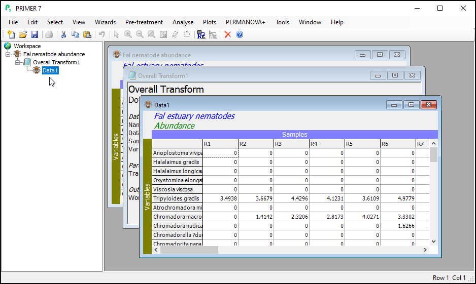
- To perform an overall transformation of the data (i.e., on all variables), click Pre-treatment > Transform(overall)....
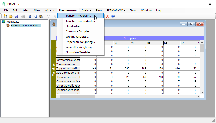
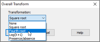
- In the 'Overall Transform' dialog box, choose (Transformation: Fourth root), then click OK.
You should now see the transformed dataset (called 'Data1') as the 'active window' in the PRIMER workspace. Note that the transformed datasheet has inherited all of the properties, factors and indicators that were associated with the original data as well.
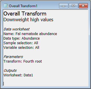
You will also see a small file (called 'Overall Transform1'), indicated by a little notepad ( ) in the Explorer tree. This shows a little more information regarding the choices you made for this particular run of the 'Transformation(overall)...' routine.
The 'active window'
The active window is identified by slightly darker shading of its border within the PRIMER workspace. Its name is also shaded in the Explorer tree. When you want to run any particular routine in PRIMER, you will need to make sure that the correct dataset (or resemblance matrix) is the active window when you launch that routine.
Notice that, although the transformed data ('Data1') is output as the active window after you do a transformation, the original datasheet is still in your workspace, and you can navigate back to it either by clicking on it's name in the Explorer tree (look right under the word 'Workspace' for 'Fal nematode abundance'), or by clicking on the window containing the datasheet itself inside the PRIMER workspace.
Re-name the transformed data
It is good practice to rename the datasheet corresponding to the transformed data for future reference within this workspace as you proceed with your work.
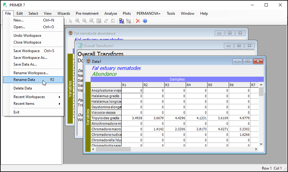
To re-name the datasheet within PRIMER, click on File > Rename Data.
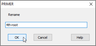
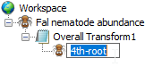
In the dialog box, type the new name you want to call it (in this example, we could re-name the sheet containing transformed data as '4th-root', as shown below), then click OK.
Alternatively, you can simply click and hover over the word 'Data1' in the Explorer tree window, and you will be able to change the name in situ right there, viz:
Before heading on to Step 2, you can optionally also now click on File > Save Workspace to save your full workspace thus far (you could use the name 'Fal_Workspace.pwk', for example).
Step 2: Resemblance
For a description of the Bray-Curtis resemblane measure and the rationale for its use with biotic data, see Clarke et al. (2006) and Chapter 2 in 'Change in Marine Communities'.
- With the data sheet named '4th-root' from the previous step as the active window, click on Analyse > Resemblance...
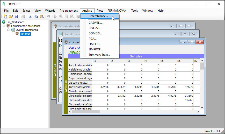
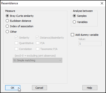
This dialog has a host of choices for you to consider, which you can uncover by clicking on the '$\bullet$Other' radio button. See Clarke et al. (2006) and chapter 7 in Legendre & Legendre (2012) for more details regarding the available choices here. For this example, however, we are going to use the Bray-Curtis resemblance measure. (This is the default for data of type 'Abundance').
- In the 'Resemblance' dialog, under 'Measure', click on $\bullet$Bray-Curtis similarity (the default), then click OK.
You will see the resulting (lower triangular form of the) matrix of Bray-Curtis similarities between every pair of samples (called 'Resem1').
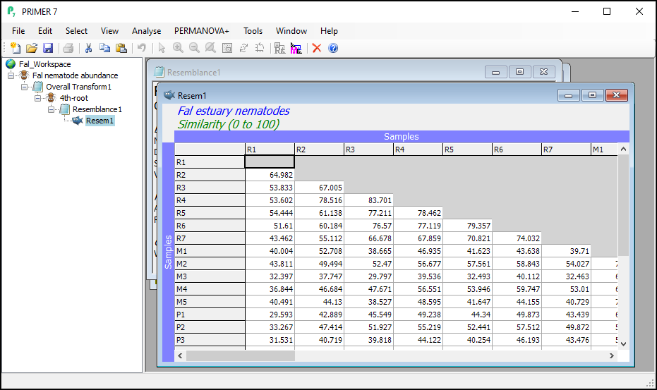
Notice that this will inherit relevant properties and also factors that were associated with the dataset from which it was generated. From the 'Resem1' matrix as the active window, click on Edit > Properties to see the properties associated with this resemblance matrix (shown below); you can also click on Edit > Factors to see the factors (which have not changed).
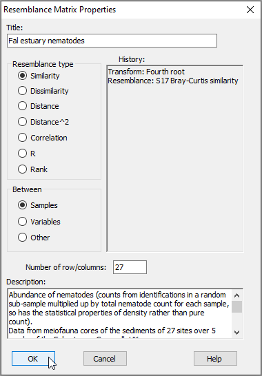
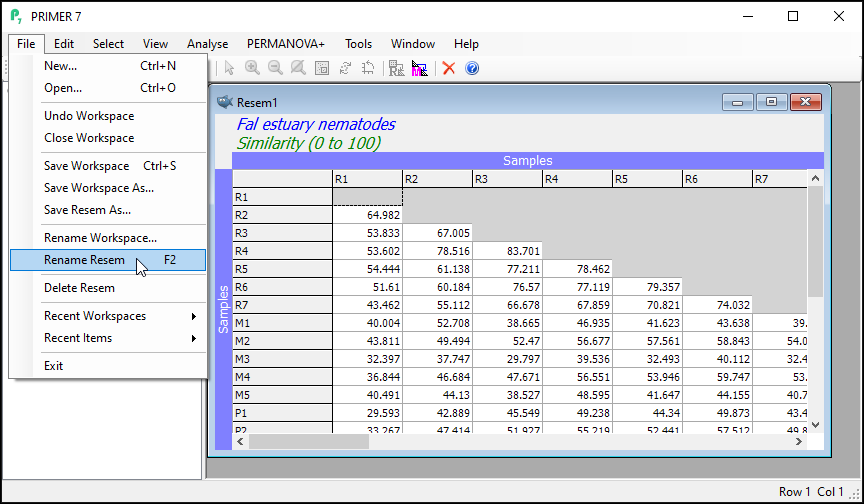
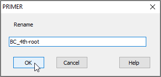
- It is (once again) good practice to re-name the sheet containing the resulting resemblance matrix (currently called 'Resem1') something that would be more useful for future reference. Click on the 'Resem1' sheet, then click on File > Rename Resem and call it 'BC_4th-root' for clarity in ensuing analyses.
Step 3: Cluster
Now that we have a resemblance matrix, we can proceed with a cluster analysis of the data. The purpose of a cluster analysis is to join together samples that are similar to one another, and also to clarify separations of groups (or clusters) of samples that may be dissimilar ( Clarke (1993) , Legendre & Legendre (2012) ). For descriptions of the clustering methods in PRIMER, see Chapter 3 in 'Change in Marine Communities'. The starting point for cluster analyses in PRIMER is always the resemblance matrix that quantifies inter-sample (or inter-variable) (dis)similarites.
Perform the cluster analysis
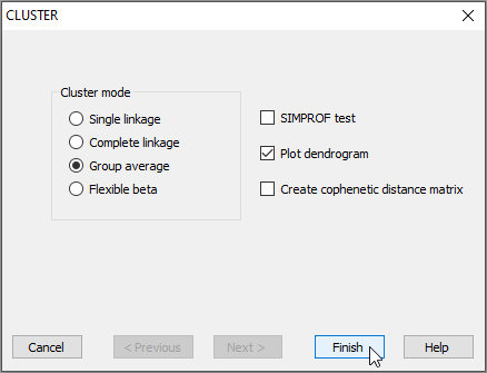
- In the PRIMER workspace file containing the Fal nematode data, click on the resemblance matrix of Bray-Curtis similarities calculated from fourth-root transformed data (called 'Resem1', or re-named to 'BC_4th-root' in the Explorer tree) to make it the active window, then click on Analyse > Cluster > CLUSTER....
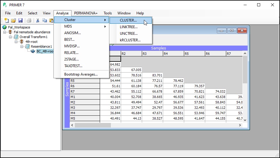
- To perform hierarchical agglomerative clustering with group-average linkage (also sometimes referred to as 'unweighted pair group method with arithmetic mean' or UPGMA), retain all of the defaults in the 'CLUSTER' dialog and click Finish.
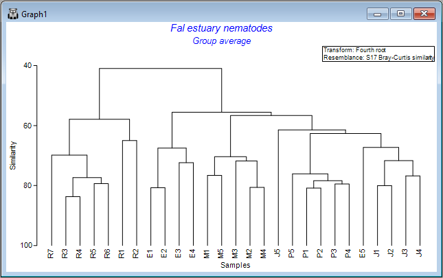
You will see an output file that provides all of the details of the clustering algorithm's pathway (shown as 'CLUSTER1' in the Explorer tree). A dendrogram will also appear as output in a new graphics window (shown as 'Graph1' in the Explorer tree), viz:
Customize the dendrogram graphic
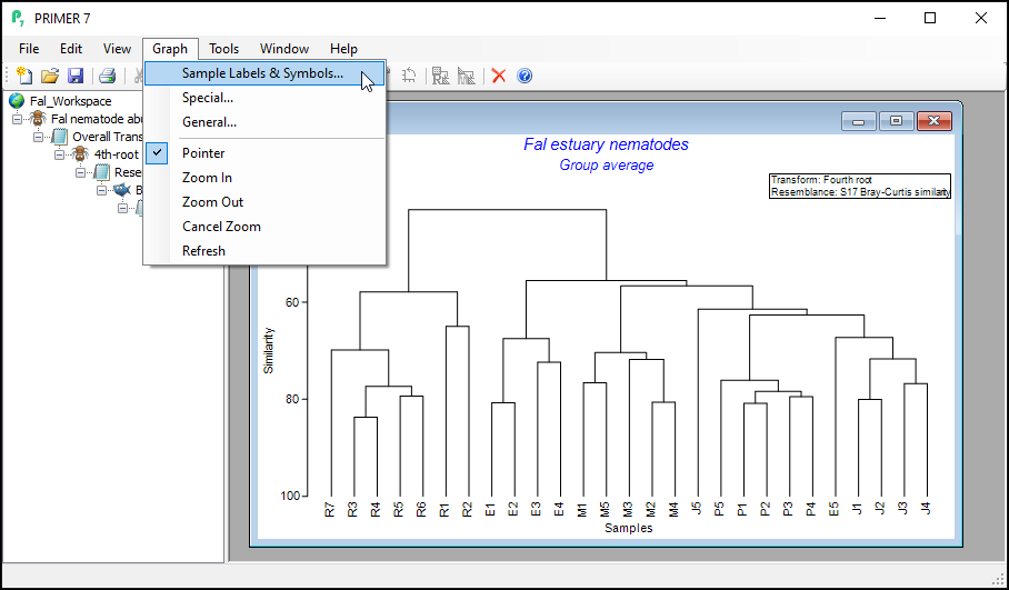
You can do a number of customizations to the dendrogram graphic.
- With the dendrogram as the active window, click on Graph and you will see a range of options.
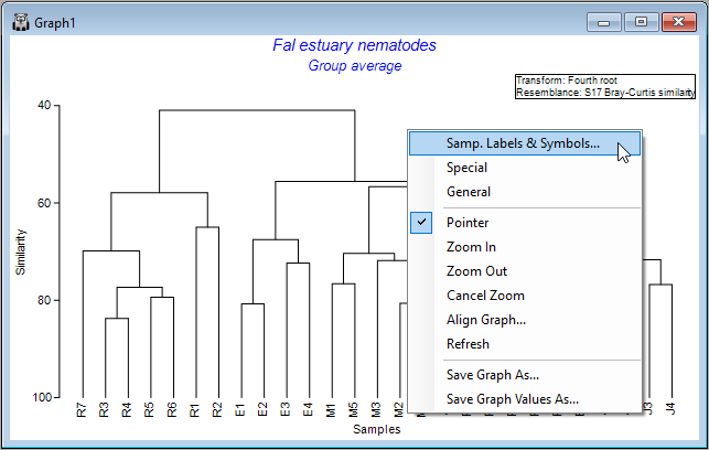
Alternatively, you can right-click anywhere inside the dendrogram's graphic window itself and a similar list pops up, along with additional options for saving the graphic (or graph values) as a separate file, etc. Note that you can also save any graph by clicking on File > Save Graph As... with the graphic you want as the active window.
The choices of Graph > Sample Labels & Symbols... and also Graph > General... will show you a set of options for changing elements that are common to all (or most) graph types in PRIMER (i.e., things like scales and labels to use for the x and y axes, titles and sub-titles, fonts, symbols, colours, etc.) In contrast, the choice of Graph > Special.. will provide a special menu of graphical options specific to that particular type of graph - in this case, a dendrogram.
Change labels and/or symbols
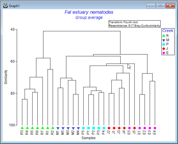
- Let's add some symbols to the plot, with the 4 creeks being represented by different symbols. Click Graph > Sample Labels & Symbols.... In the resulting 'Graph Options' dialog, under the 'Samp. labels & symbols' tab, choose (Labels $\checkmark$ Plot) & (Symbols $\checkmark$Plot & $\checkmark$By factor Creek), then click OK.
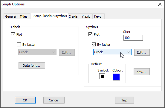
Note that the 'Samp. labels & symbols' dialog will automatically offer you the option to choose labels or symbols corresponding to any factors that are associated with your resemblance matrix. Tip: For graphing purposes, it is a good idea to use short names for samples (if you can) and (more importantly) for levels of factors, so they will be easy to display on plots.
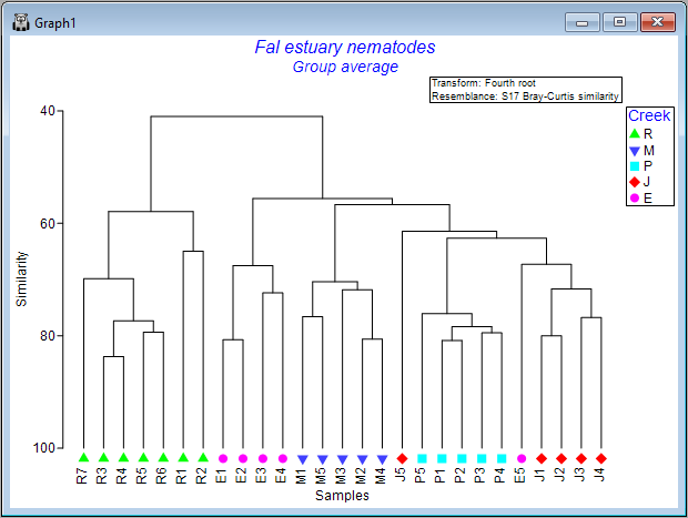
The result is a more colourful and informative dendrogram, which clearly shows a pattern of (generally) high similarity among assemblages within each of the four creeks, (similar symbols tend to be clustered together), and some clear distinctions between assemblages in different creeks, with Restronguet Creek ('R') appearing most different from the others (only about ~40% similar to other creeks, on average).
Zoom in and out
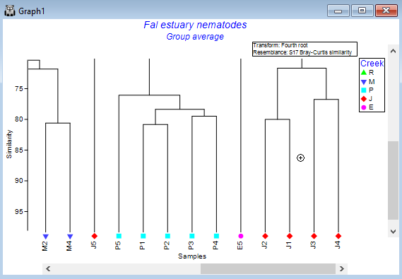
If you have a very large dendrogram with a lot of samples, it is helpful to be able to zoom in and out in order to see details present in different portions of the dendrogram.
To Zoom in, click Graph > Zoom in (or click on the 'zoom-in' icon  in the ribbon of tools shown under the main menu items). In zoom-in mode, your cursor will change into a little 'plus' symbol
  when poised over your graphic, and with this you simply click on the dendrogram to zoom in on that area. Click multiple times to continue zooming in.
To Zoom out, click Graph > Zoom out (or click on the little icon with a minus symbol inside a magnifying glass  ). Now the cursor changes into a little 'minus' symbol
  , and clicking on the graphic zooms you back out again.
To cancel the zoom entirely (to see the entire dendrogram again), click on Graph > Cancel Zoom (or click on the cancel-zoom icon  ).
).
Collapse nodes to simplify
Another option, if you have a very large dendrogram, is to simplify the view by clicking on any one of the vertical branches. This will collapse all of the samples under that branch into a single entity, making it easier to see patterns in what remains. For example, click on the vertical branch that leads to all of the samples from Restronguet Creek ('R'), and the dendrogram will look like this:
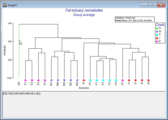
Simply click on that same vertical branch again to toggle that 'collapse' option off, and you will see all of the individual samples within that node again in the full dendrogram, as before.
Rotate leaves around the nodes
It is important to remember that the dendrogram should be thought of like a 'mobile', dangling from a ceiling. In this way, the leaves dangling from each node can be rotated around the node. Thus, the specific ordering of the samples you see in the dendrogram, while being constrained by it in some way, has a bit of flexibility: sample units can be rotated around the nodes.
To explore this flexibility visually, click on any horizontal line of the dendrogram, and you will see its leaves will 'flip', accordingly. Clearly, quite a lot of re-arrangements of the sample ordering provided in the initial output are possible, so it is often useful to experiment with this a bit to achieve an ordering that may be most useful for interpretation of relationships/clusters.
For example, one possible re-ordering looks like this:
Change the orientation
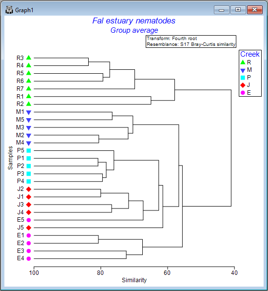
The default output orientation for a dendrogram in PRIMER is to have the hierarchical agglomeration going 'Up' (i.e., individual sampling units hang downwards); however, you can customise its orientation. For example, for the Fal estuary nematodes, click on Graph > Special..., then in the 'Dendrogram Options' dialog box, under 'Orientation', choose $\bullet$Right, and click OK.
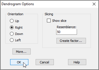
This yields the following:
 .
.
Step 4: Ordination
The cluster analysis goes some way towards helping us to understand potential patterns of similarity among the samples. It is particularly good at showing us clusters of samples that are highly similar. To better visualise patterns of relationships among all of the samples simultaneously, we can use methods of ordination. In particular, non-metric multi-dimensional scaling (nMDS) is a wonderfully robust tool for visualising high-dimensional systems on the basis of a chosen resemblance measure ( Kruskal & Wish (1978) ; Clarke (1993) ). Non-metric MDS essentially places points into an arbitrary Euclidean space of set dimension (typically producing a 2D or 3D plot) so as to preserve, as well as possible, the rank-order of the dissimilarities between pairs of samples. For more details on multi-dimensional scaling, see Chapter 5 of 'Change in Marine Commmunities'.
Create a non-metric MDS plot
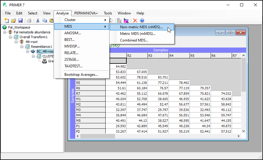
From the Bray-Curtis resemblance matrix ('BC_4th-root' in this example), click Analyse > MDS > Non-metric MDS..., then click OK to run the MDS algorithm with all of the default options.
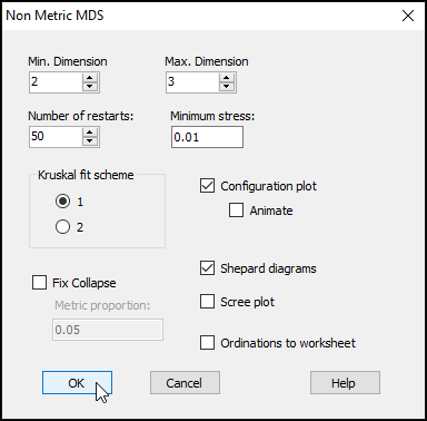
The resulting 'Multi-plot1' output graphic gives you 4 individual plots (in a 2-by-2 array), as follows:
- the best 2D solution (from 50 random starts)
- the Shepard diagram for the best 2D solution
- the best 3D solution (from 50 random starts); and
- the Shepard diagram for the best 3D solution
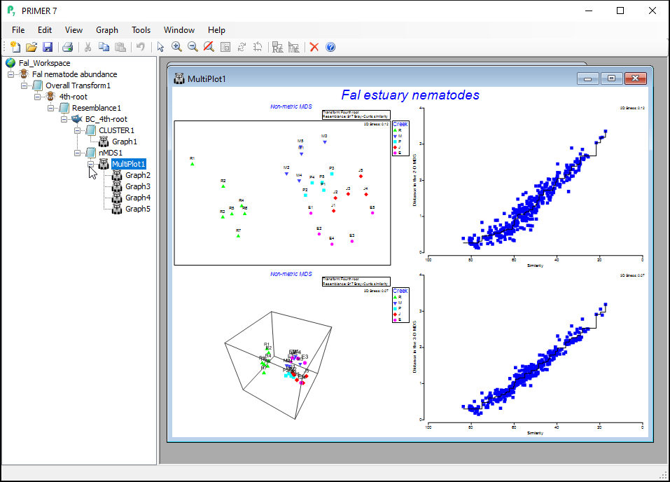
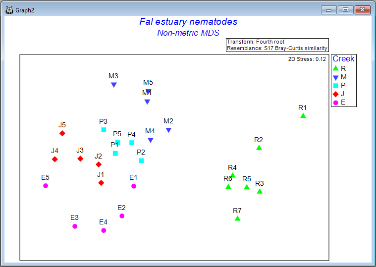
Clicking on the '+' symbol next to the word 'MultiPlot1' in the Explorer tree reveals the four graphics that comprise this multi-plot object ('Graph2', 'Graph3', 'Graph4', 'Graph5'). If you then click on 'Graph2' in the Explorer tree, or if you click in the Multi-plot itself on the plot in the upper left-hand corner, you will see a single graphic now; namely the best (lowest-stress) 2-dimensional non-metric MDS plot for the Fal estuary nematodes.
Interpretation
The plot does not have x and y axes, as the scale here is arbitrary. The non-metric MDS algorithm attempts only to preserve rank-order dissimilarities, so interpretations are restricted to relative distances among points in the plot. For example, we can make statements like: "The dissimilarity between sample R7 and M3 appears to be larger than the dissimilarity between sample M3 and M2", but we cannot tell (directly from the plot) what the specific sizes of those particular dissimilarities are.
It is clear from this output that Restronguet Creek ('R') has assemblages of nematodes that are quite dissimilar from those found in the other four creeks. That's consistent with what we saw in the cluster analysis of these data. We can, however, get quite a few more insights from the nMDS plot than were apparent in the cluster dendrogram. For example, relationships among the assemblages from the other four creeks seem to be ordered (from the bottom-left towards the top of the plot) as follows: Percuil → St. Just → Pill → Mylor. It is also apparent that the samples from Pill Creek ('P') form a tighter cluster hence are not as variable as the samples from (say) Restronguet Creek ('R'), which are more spread out. Being able to see potential gradients of change in assemblages, the degree of between-group differences, as well as the relative sizes of within-group dispersions, is all very useful.
Step 5: ANOSIM test
The ordination plot gives us a visualisation of the rank-order relationships among the samples, based on the dissimilarity measure. Next, we may wish to test the null hypothesis that there are no differences among the five creeks. We can use a non-parametric multivariate permutation test called analysis of similarities (ANOSIM, Clarke (1993) ) for this test. For more details on the ANOSIM test, see also Chapter 6 in 'Change in Marine Communities'. We will be doing a one-way ANOSIM test here (as there is a single factor in this example); for more information on multi-way designs with ordered and/or unordered factors, see Somerfield et al. (2021a) , Somerfield et al. (2021b) and Somerfield et al. (2021c) .
Perform the ANOSIM test
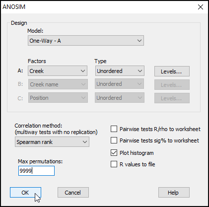
From the Bray-Curtis resemblance matrix (called 'BC_4th-root' in this example), click on Analyse > ANOSIM... and you will see the ANOSIM dialog.
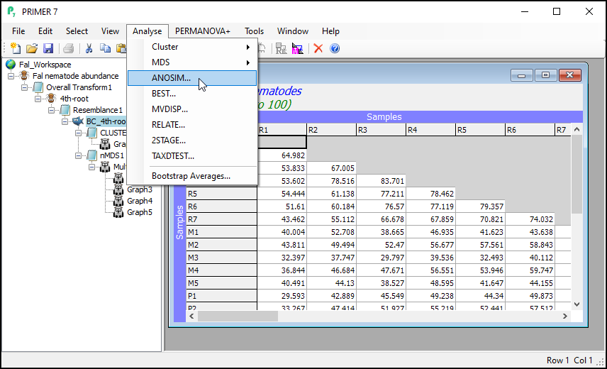
Here, we are performing a one-way ANOSIM (there is just one factor whose levels are un-ordered), so we can leave most of the defaults in the dialog as they are. We should, however, increase the permutations to a larger value, so change the 'Max permutations' from the default value of 999 to 9999, then click 'OK'.
The results, including the overall ANOSIM test for differences among all groups, as well as the ANOSIM tests of all pair-wise comparisons, are provided in the output file called 'ANOSIM1'. The overall test is clearly highly significant, with R = 0.816 and a significance level of 0.01%. This corresponds to a p-value of P = 0.0001 (the smallest possible value attainable for 9999 permutations). Note that, in PRIMER, all p-values are reported for ANOSIM tests as 'significance levels', expressed as a percentage. For example, a p-value of P = 0.0619 would be given in the output file as a significance level of 6.19%.
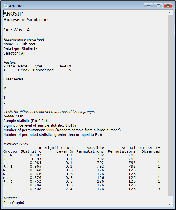
The full set of pairwise tests is performed, and the strength of the differences between any pair of groups is well captured by the relative sizes of the R statistic - larger values indicate groups that are more different (more distinct or more easily distinguishable) from one another. The comparison of assemblages from St Just Creek (J) vs Percuil Creek (E) has the lowest R statistic (R = 0.508) of any tests done in this example, although this difference is still a statistically significant one (P = 0.024). Note that no 'correction' is being made here for multiple tests. The end-user is able to consider applying such a correction if desired (or may perhaps simply consider the frequency of 'significant' results obtained, given the number of tests performed), bearing in mind that each test is done using an exact permutation algorithm in order to generate the individual significance levels produced in the output, ignoring all other tests.
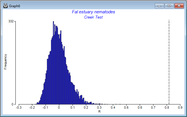
Also provided as output ('Graph6') is a histogram showing the distribution of values of the ANOSIM R statistic under permutation for the overall test. The observed value of the ANOSIM R statistic (0.816) is shown on the plot as a vertical dotted line. The purpose of the histogram is to show visually the departure of the observed value of R (or not) from the distribution of values of R expected under a true null hypothesis of 'no difference' among the groups.
Summary of the pathway
A summary of the essential routines in PRIMER that were used to produce the 5-step analysis pathway described above for the nematode (biotic) data from the Fal estuary is given in the table below:
| Step | To implement in PRIMER: |
|---|---|
| 1. Fourth-root transformation | From the original data sheet: click Pre-treatment > Transform(overall) > (Transformation: Fourth root), click OK. |
| 2. Bray-Curtis resemblance | From the transformed data sheet: click Analyse > Resemblance > (Measure $\bullet$Bray-Curtis similarity) & (Analyse between $\bullet$Samples), click OK. |
| 3. Hierarchical group-average cluster analysis | From the resemblance matrix: click Analyse > Cluster > CLUSTER... > (Cluster mode $\bullet$Group average) & ($\checkmark$Plot dendrogram), click Finish. |
| 4. Non-metric MDS ordination | From the resemblance matrix: click Analyse > MDS > Non-metric MDS (nMDS)... > (see if you are happy with the default settings), click OK. |
| 5. Analysis of similarities (ANOSIM) | From the resemblance matrix: click Analyse > ANOSIM... > Design > (Model: One-Way - A) & Factors > A: Creek) & (Max permutations: 9999) & ($\checkmark$Plot histogram), click OK. |
6. Some Wizards
Basic multivariate analysis
A useful analysis pathway (including the Example Analysis Pathway done above, with its five steps), can be accomplished in one fell swoop using the Basic multivariate analysis wizard. This will perform a suite of multivariate analyses commonly performed for either biotic or environmental data types, with options available that match the typical choices made for handling these different types of data.
Run the 'Basic multivariate analysis' wizard
Let's suppose you wanted to repeat the step-by-step analyses we did before, but this time using a different pre-treatment option. For example, you may decide you'd like to analyse the same data using presence/absence information only, so as to emphasise only the turnover in species identities (and not differences in abundance values) across sample units. It would be great to run this whole set of analyses quickly, rather than going through them again one at a time.
Click on the original 'Fal nematode abundance' datasheet in the Explorer tree and then click Wizards > Basic multivariate analysis....
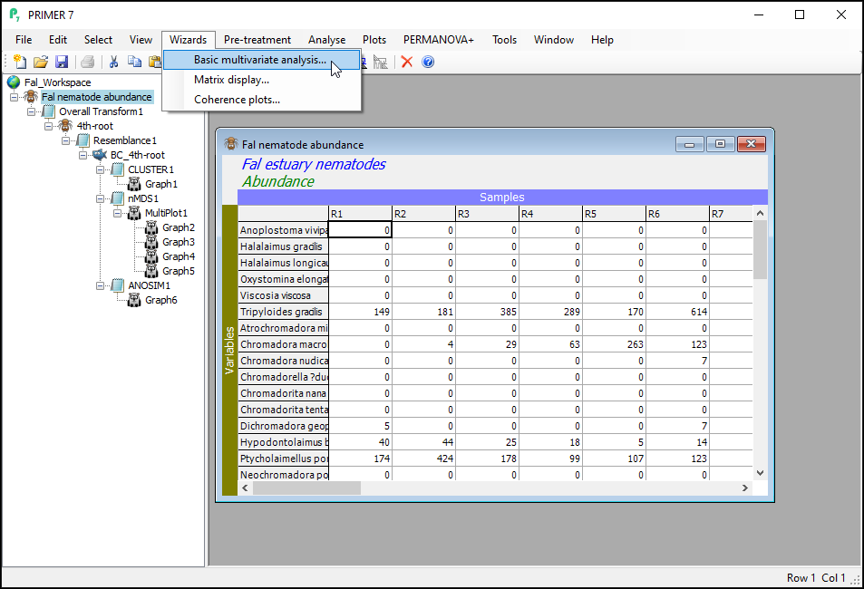
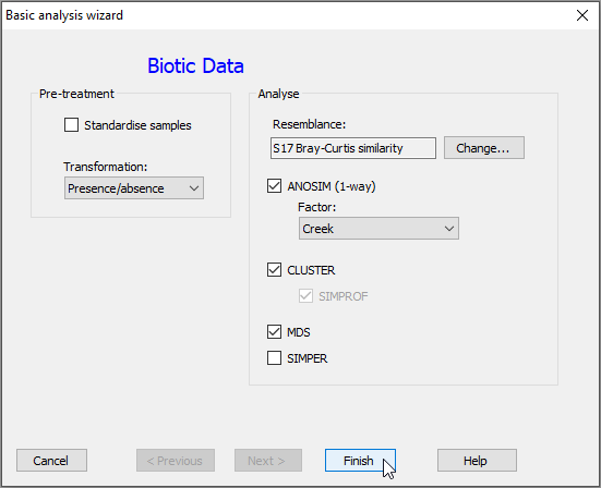
In the dialog box that follows, we can see that PRIMER is offering to perform a suite of basic multivariate analyses that are commonly performed for 'Biotic Data' (shown in bold blue font at the top). You can choose from a couple of (common) pre-treatment options, and then it will perform the analyses you choose (via the relevant checkboxes under 'Analyse'), using the default options for each routine. Note that different options would be shown for data of a different type (e.g., for environmental data). Recall that the 'type' of data is specified by you when you import the data into PRIMER. This can be changed for a given data sheet by clicking on Edit > Properties at any time.
Under 'Pre-treatment', choose 'Transformation: Presence/absence' and under 'Analyse', leave all of the default options, except you can untick the checkbox next to the 'SIMPER' routine (for now), then click Finish.
All of the requested analyses are done, and the resulting output files and graphics are shown in the Explorer tree window. Click on any of the items in the Explorer tree to see the steps that were taken, including specific data sheets, resemblance matrices, graphical outputs and results files. Although you will generally use PRIMER to perform individual analyses, one routine at a time, this wizard provides a quick way to achieve multiple analyses (provided you know a priori that you want to do them) with a single stroke.
The ANOSIM results ('ANOSIM2') and the 2D nMDS output (Graph9) obtained by this run of the wizard are shown below:
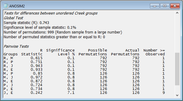
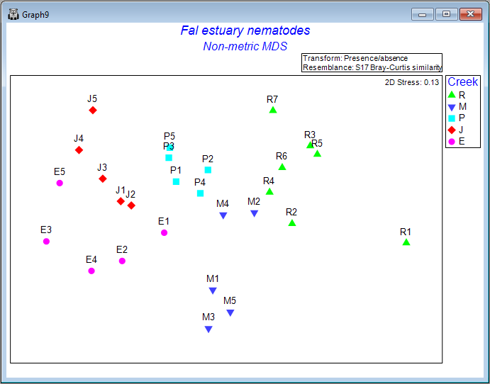
In this example, we can see that there are statistically significant differences in the identities of nematode species among the five creeks (ANOSIM R = 0.743, P = 0.001 with 999 permutations), although the pattern in the nMDS plot suggests that the difference between Restronguet Creek and the other creeks is not as great as what was observed when abundance information was included in the Bray-Curtis calculation. (Compare 'Graph9', as shown above, with 'Graph2' that we obtained earlier.)
Expanding and collapsing the Explorer tree
Note that this new set of analyses, performed using the wizard on the original imported data, will initiate its own new branch of the Explorer tree. You can always initiate a new analysis starting from a given item in the tree (e.g., from a data sheet or a resemblance matrix, etc.), and the tree will expand, generating a new branch, to accommodate these new analyses. You can use the '+' and '-' symbols in the Explorer tree to 'roll up' or 'unpack' the items in the tree belonging to a particular branch at any time.
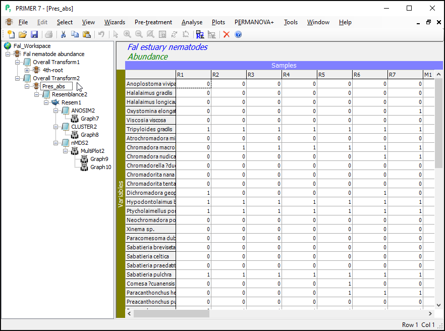
For example, clicking on the '-' symbol next to the item named '4th-root' will 'roll up' all of the items associated with our original analysis (based on a fourth-root transformation), so the analyses that were done by the Wizard (based on presence/absence) are now closer to the top of the Explorer tree window. For clarity, we might choose to rename the sheet called 'Data1' (the data sheet produced by the wizard after performing the presence/absence transformation) to 'Pres_abs'.
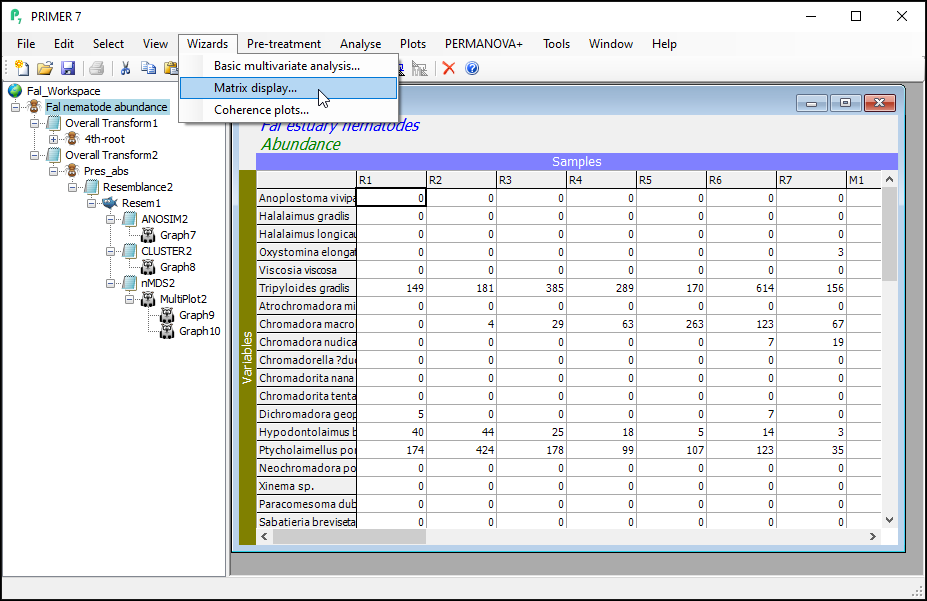
Matrix display
The Matrix display wizard produces a shade plot of a multivariate data matrix, with a useful ordering of its rows and columns that can help to clarify inter-sample and inter-species relationships, as well as gradients in turnover based on a resemblance matrix of choice.
Create a Matrix display
Click on the original data sheet ('Fal nematode abundance', at the top of the Explorer tree window), then click on Wizards > Matrix display....
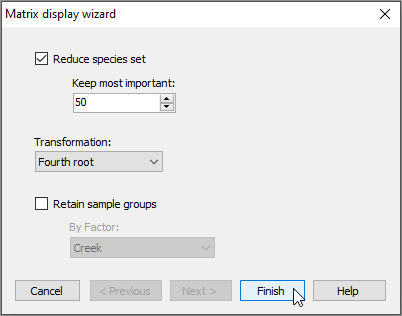
In the 'Matrix display wizard' dialog, leave the defaults, but choose (Transformation: Fourth root), then click Finish.
The default graphic ('Graph13')shows a shade plot of the 50 most important species (here, 'most important' is defined based on the percent(%) of the total abundance obtained by a species in any sample). Each value in the data matrix is represented by a shaded rectangle (from white to black, by default), where the degree of shading corresponds to the abundance values (after fourth-root transformation), as shown in the key (in this example, the transformed data values range from 0 to 8).
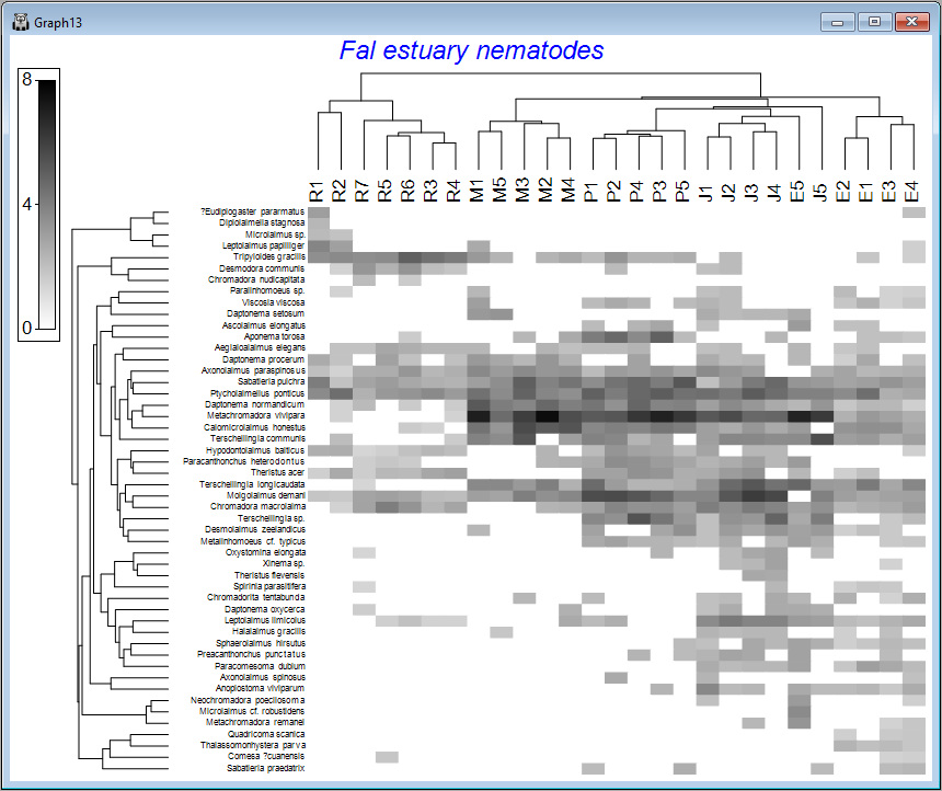
Here, samples are ordered so as to maximise their concordance with a model of 'seriation' (or turnover), defined on the basis of Bray-Curtis similarities calculated on fourth-root transformed data. They are (furthermore) constrained according to a dendrogram constructed from a hierarchical group-average cluster analysis of those similarities ('Graph12' in the Explorer tree). The species, in turn, are ordered according to a model of seriation based on an Index of Association calculated among species after first standardising the species variables by their total abundance. They are (similarly) further constrained by their own cluster dendrogram ('Graph11' in the Explorer tree).
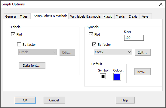
It would perhaps be helpful to see the different creeks as different symbols on this plot. With Graph13 (the shade plot itself) as the active item in the Explorer tree, click Graph > Sample Labels & Symbols, then choose (Labels $\checkmark$Plot) & (Symbols $\checkmark$Plot > $\checkmark$By factor Creek) and click OK.
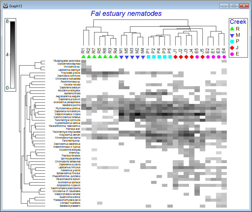
We can see from the above image that some creeks contain a rather different set of species and/or different abundances of the same species. The ordering of whole creeks shown in the shade plot (obtained using the 'seriation' model) reflects the ordering we saw in the nMDS plot for these creeks as well (see the page 'Step 4. Ordination').
From a matrix display (or shade plot), clicking on Graph > Special reveals a very large number of colours and other graphical options and parameters allowing the user to alter and enhance this graphic for their purposes. These are too numerous to describe in detail here, but they include a host of methods for sorting the rows and/or columns (i.e., by clicking on the Reorder... button in the Graph > Special dialog).
7. Run a PERMANOVA
Overview
If you have purchased the PERMANOVA+ add-on, then you will have an additional menu item that allows you to perform a broad range of additional analyses using a suite of routines that are not available in the base PRIMER 7 package, including PERMANOVA, PERMDISP, PCO, DISTLM/dbRDA and CAP. See the PERMANOVA+ user manual for details regarding these routines and the underlying methods.
Here, we will run through a quick example of how to set up and run a multi-factor PERMANOVA analysis in PRIMER. Permutational multivariate analysis of variance (PERMANOVA) partitions variation in the space of a chosen dissimilarity measure in response to one or more factors in a specified sampling protocol or experimental design ( Anderson (2001a) , Anderson (2017) ). Tests of individual terms in a PERMANOVA model are achieved by constructing correct (pseudo-)F ratios on the basis of expectations of mean squares (EMS), and p-values are obtained using correct permutation algorithms given the full study design.
Importantly, the PERMANOVA routine in PRIMER allows the user:
- to specify whether factors are fixed or random,
- to specify whether a factor is nested in one or more other factors,
- to test interaction terms,
- to include one or more quantitative covariates in the analysis,
- to remove individual terms from a model or to perform pooling,
- to handle correctly:
- mixed models
- user-specified contrasts
- BACI designs (before-after/control-impact),
- asymmetrical designs (e.g., in environmental impact studies),
- randomised blocks,
- split plots,
- hierarchical designs,
- repeated measures,
- unbalanced designs (Type I, II or III sums of squares),
- ... and more.
A three-factor hierarchical design
We will run PERMANOVA on an example dataset consisting of assemblages of molluscs collected from holdfasts of the kelp Ecklonia radiata in a 3-factor hierarchical experimental design. There were n = 5 holdfasts collected from each of 2 areas (tens of meters apart) at each of 2 sites (hundreds of meters to kilometers apart) from each of 4 locations (hundreds of kilometers apart) in rocky reef habitats along the northeastern coast of New Zealand ( Anderson et al. (2005a) , Anderson et al. (2005b) ).
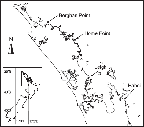
The map above shows the four locations on the northeastern coast of New Zealand from which holdfasts were collected for the study: Berghan Point, Home Point, Leigh and Hahei (reproduced from Fig. 1 in Anderson et al. (2005a) ).
The example data are found in the file called NZ holdfast fauna abundance.pri in the folder named 'NZ holdfast fauna' inside the 'Examples v7' folder that can be downloaded by clicking Help > Get Examples V7.... There were 351 taxa (rows) from 15 different phyla quantified in this study. Here, we shall focus only on the phylum Mollusca (105 taxa).
Our interest lies in quantifying the degree of turnover in the identities of mollusc species at different spatial scales, as measured by the Jaccard resemblance measure. This a fully hierarchical sampling design with three spatial factors, as follows:
- Locations (random with 4 levels: Berghan Point, Home Point, Leigh and Hahei)
- Sites (random and nested in Locations, with 2 sites per location)
- Areas (random and nested in Sites, with 2 areas per site)
Areas are therefore also (necessarily) nested in Locations as well.
Steps in a PERMANOVA analysis
The two essential steps required to run a PERMANOVA analysis in PRIMER are always:
- first, specify the design; and
- then, run the PERMANOVA analysis, given the design, on a chosen resemblance matrix (arising from the data of interest).
Generally, we first need to get our data in to PRIMER, perform appropriate pre-treatment(s), if any, then calculate a resemblance matrix from this. A resemblance matrix will always serve as the starting point for any PERMANOVA analysis.
An analysis of only the mollusc species from the holdfasts in accordance with the three-factor hierarchical design, based on Jaccard resemblances, will follow the following steps:
- Open the example data file in the PRIMER workspace. Select a subset of the variables corresponding to only the mollusc species for what follows.
- Calculate Jaccard similarities* among the sampling units (individual holdfasts).
- Specify the experimental/sampling design (creating a design file).
- Run the PERMANOVA routine (partitioning and p-values via permutation for each term in the model.
- Do an ordination of distances among centroids to visualise the effects and the relative importance of the factors.
(*Note: the Jaccard resemblance measure utilises only presence/absence information, so we do not need to perform a pre-treatment transformation step for this example.)
Step 1: Data selection
Open up the example data file
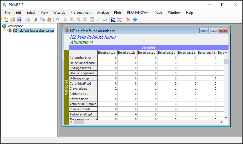
Launch PRIMER, then click File > Open... from the main menu, navigate to the folder named 'NZ holdfast fauna' in the 'Examples v7' directory, and select 'NZ holdfast fauna abundance.pri'. Click Open to display the species matrix.
Click on Edit > Indicators... and you will see that the data includes information about whether individual taxa were counted (enumerated) or quantified on an ordinal scale ('Ordinal' = 'N' or 'Y', respectively). Also shown are indicators showing the taxonomic groups in which each species (or taxon) variable belongs, with different levels of the taxonomic hierarchy being provided as different indicators (i.e., 'Genus', 'Family', 'Order', 'Class' and 'Phylum').
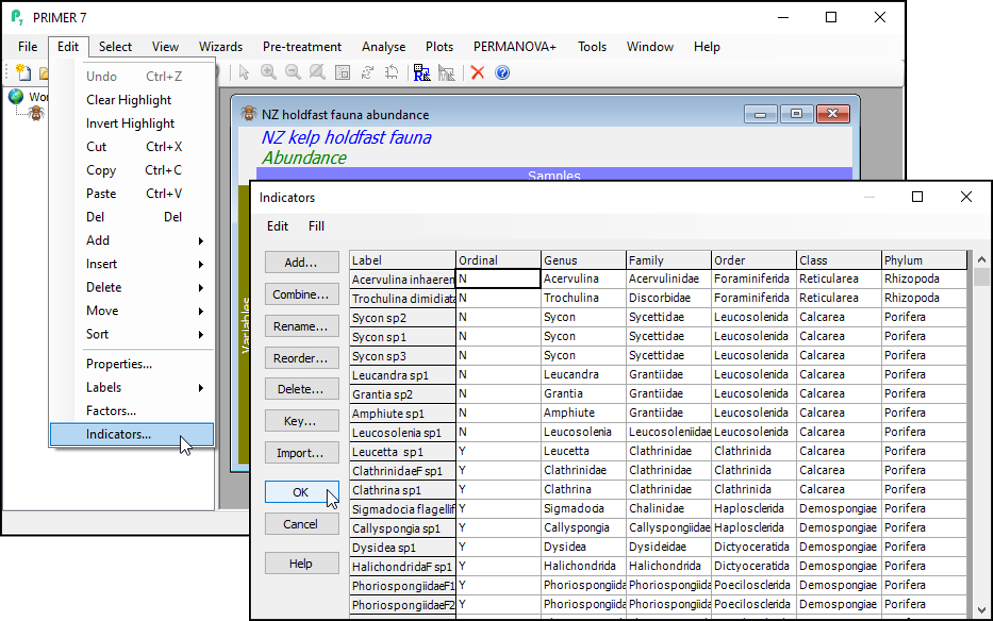
Click OK on the 'Indicators' dialog, so the data matrix is the active item in the workspace again.
Select a subset of variables, using an indicator
We wish to select just the mollusc species for the analysis.
- From the 'NZ holdfast fauna abundance' data sheet, click Select > Variables...
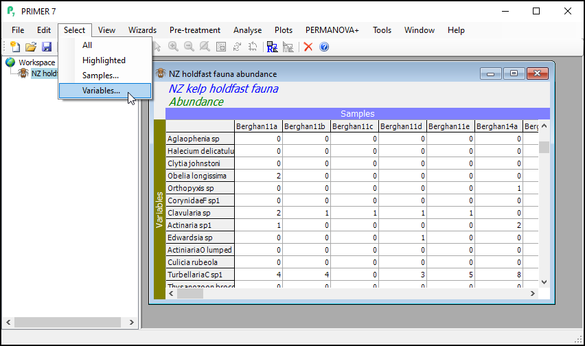
- In the 'Select Variables' dialog, choose ($\bullet$Indicator levels > Indicator name: Phylum) and click Levels....

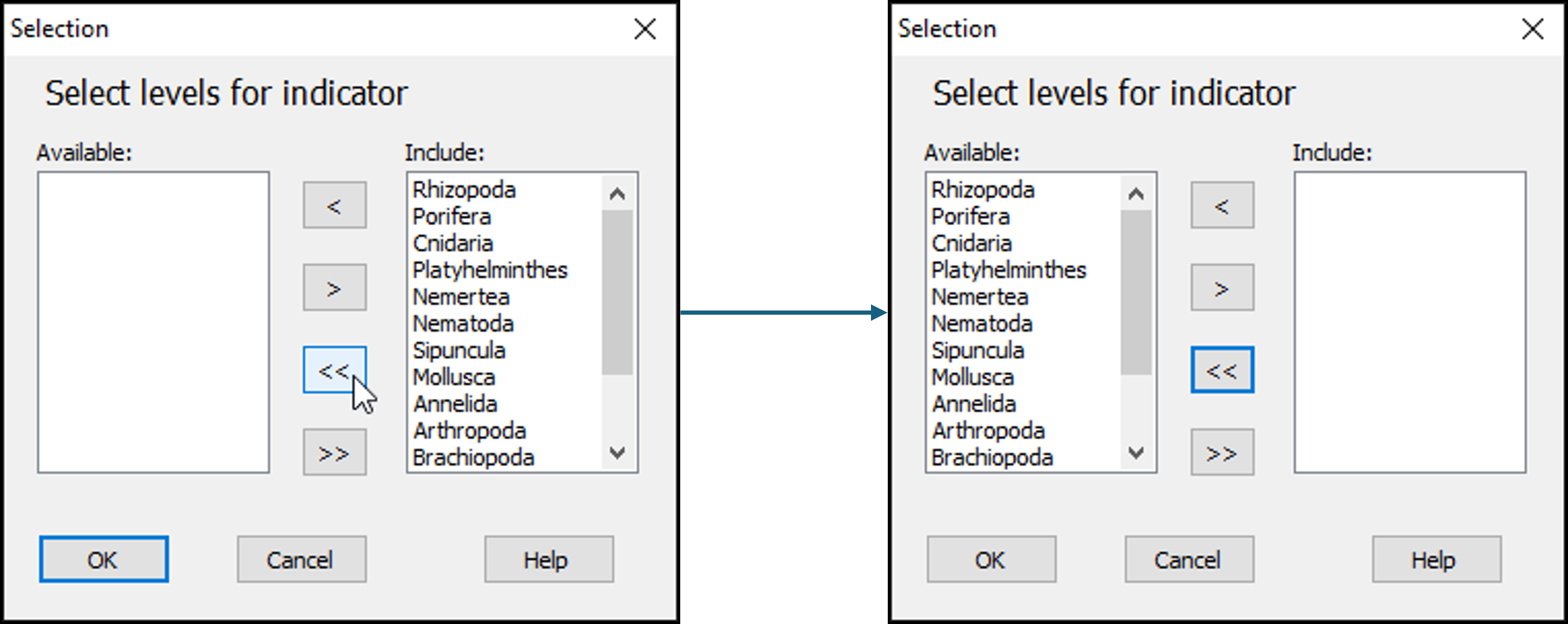
- In the 'Selection' dialog, first move all of the phylum categories from the 'Include:' box (on the right) to the 'Available:' box (on the left) by clicking on the double-left-arrow button:
 .
.
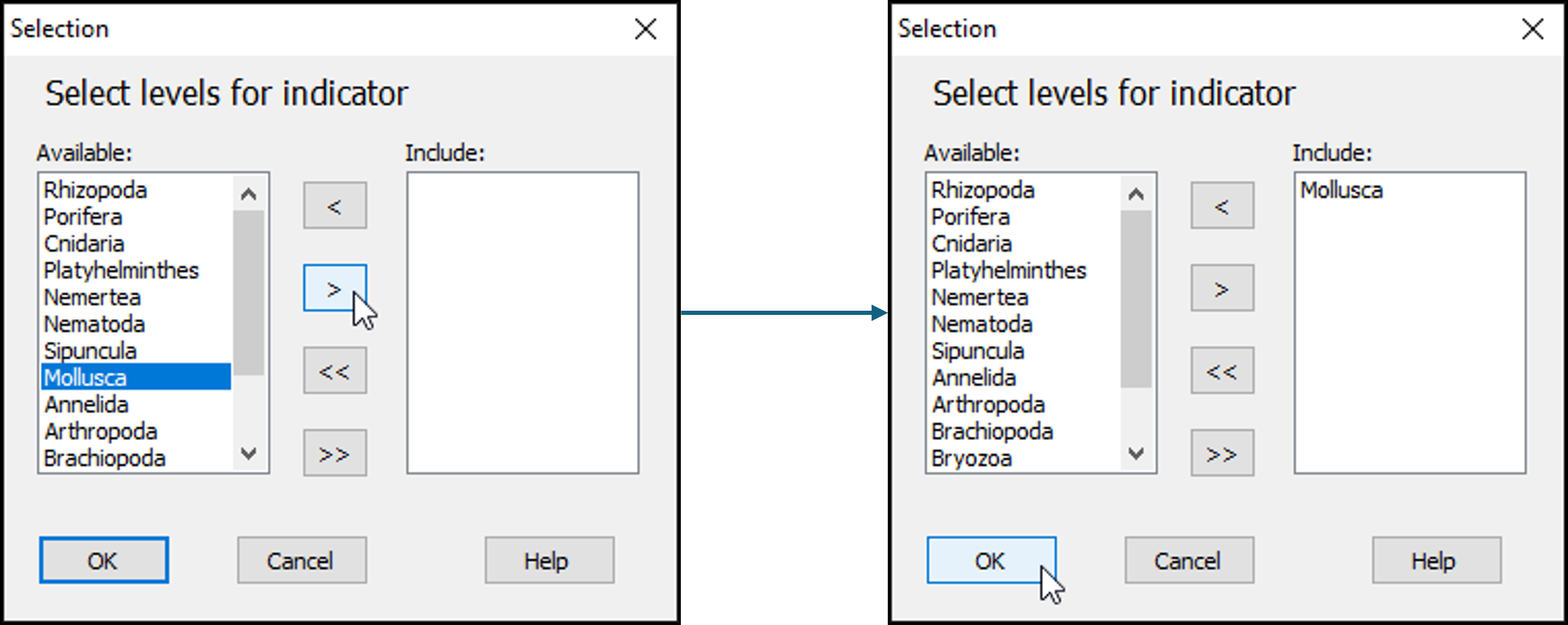
- Next, click on the word 'Mollusca' in the list of 'Available' phylum categories, and click on the single-right-arrow button:
 . This will move it to the 'Include:' box (right-hand side) of the 'Selection' dialog.
- Click OK on the 'Selection' dialog, then click OK on the 'Select Variables' dialog.
Voila! Whenever you have selected a subset of data (this might be a subset of variables, as done here, or a subset of samples, or both), then the data matrix will have a turquoise background colour to indicate that you have done this, like so:
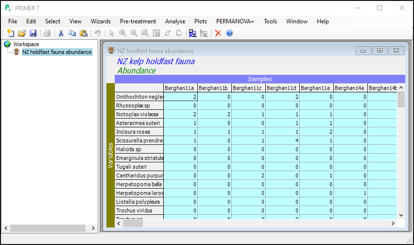
Any analyses done on a selected subset of data will only be performed on that subset. It is usually a good idea to duplicate and rename a selected subset of data, so as to keep any analysis done on that subset of data clear and separate from the (full) original dataset. Note that subsetting does not affect the original full data matrix of information in any way, which is still always there. You can clear any subset selection (of variables and/or samples) by clicking on Select > All to return to the full data matrix in its entirety. (The turquoise background colour will go away when you do that, and the formerly selected data will yet be highlighted in a purple-ish hue. Clicking on Select > Highlighted can then be used to re-instate the selection from before, if desired.)
Duplicate and rename a selected subset of data
From the subsetted data matrix, click Tools > Duplicate.
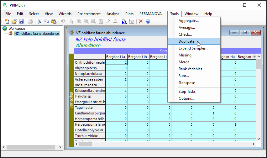
The result will be a new data sheet that contains only the subsetted data (in this case, only the molluscs). It shows up in the Explorer tree window. In the present example, this will (automatically) be called 'Data1'. It is no longer turquoise. The Duplicate routine was performed only on the subsetted (turquoise) data from the original sheet, yeilding this new data sheet, a subset of the original. If you click on Edit > Properties..., you will see that this new sheet now only has 105 variables ('Number of rows:').
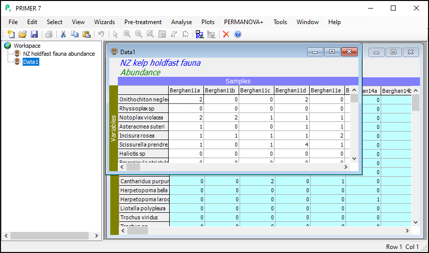
Click, hover and click again on the name 'Data1' in the Explorer tree window (or click File > Rename Data or hit the 'F2' key) and type in a new name for the subsetted data sheet: Molluscs.

At this point, you might like to save your workspace. Click File > Save Workspace As... > (Filename: NZ_holdfast_molluscs.pwk).
Step 2: Jaccard resemblance
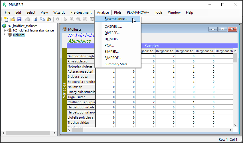
Calculate the Jaccard resemblance
From the 'Molluscs' data sheet, click Analyse > Resemblance....
In the 'Resemblance' dialog, choose ($\bullet$Other) and then click on the drop-down menu to find 'S7 Jaccard', then click OK. (Note: 'S7' refers to the nomenclature used by Legendre & Legendre (2012) in their Chapter 7 on measures of ecological resemblance).
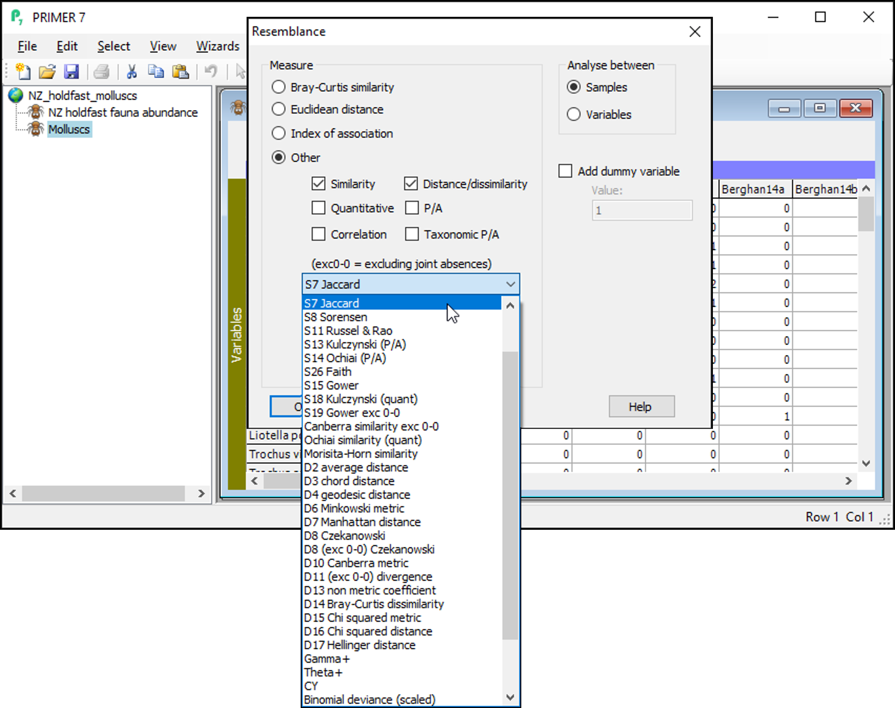
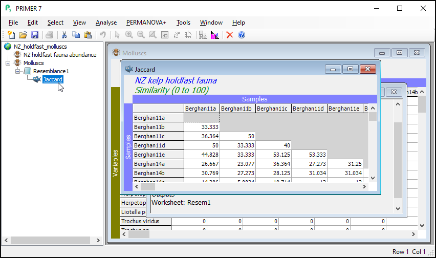
This produces a Jaccard similarity matrix among all pairs of holdfasts, called 'Resem1' by default. A nice feature of the Jaccard similarity measure is that it is directly interpretable as the percentage of shared species. For example, the first two holdfasts in the data matrix have a Jaccard similarity of 33.33%, so approximately one-third of the species that occur in either one or the other holdfast occur in both of them (i.e., are jointly present).
You can re-name this 'Jaccard' (click on the name 'Resem1' in the Explorer tree and hit the 'F2' key to re-name it), for clarity in what follows.
Step 3: Specify the design
PERMANOVA requires a design file to run.
You can see the Factors associated with the holdfast data matrix (or its resemblance matrix) by clicking on Edit > Factors.... These factors will be 'visible' to the PERMANOVA dialog that we will use to create our design file.
For this study, we want to create a design file that has all of the information that PERMANOVA will need to construct the correct partitioning, the correct pseudo-F ratios and the correct permutation algorithms to test every term in the model that is implied by the design. For this example, we have a fully hierarchical (nested) study design with three random factors: Locations, Sites (within Locations) and Areas (within Sites).
- From the resemblance matrix ('Jaccard'), click PERMANOVA+ > Create PERMANOVA Design....
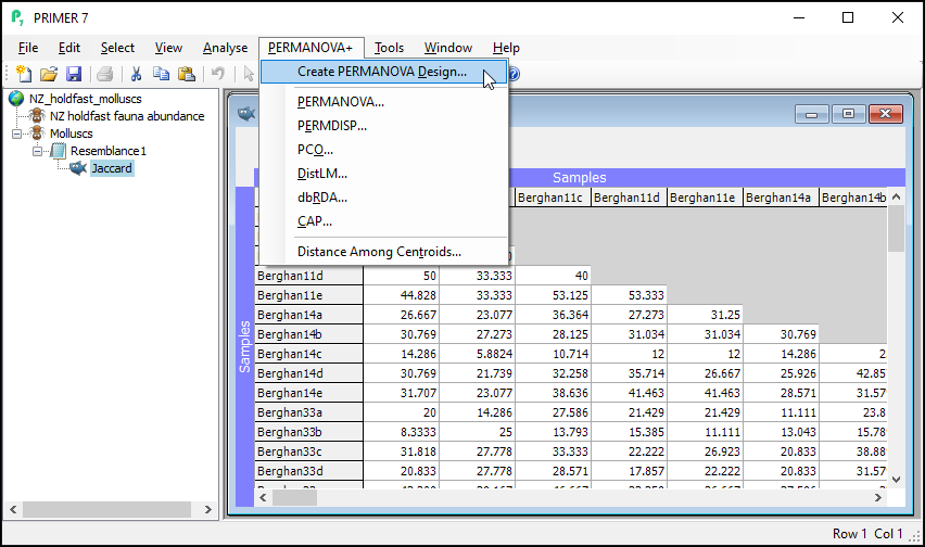
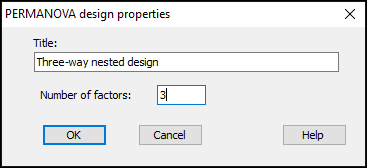
- In the 'PERMANOVA design properties' dialog, pick a title for your design file, and indicate the number of factors. For the holdfast example, we will choose (Title: Three-way nested design)&(Number of factors: 3), then click OK.
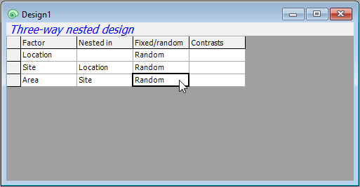
- You will see an empty design file with three rows, one for each factor. Each row will correspond to a factor in your design. You will need to specify, in turn, the name and properties of each factor for the analysis in its own row.
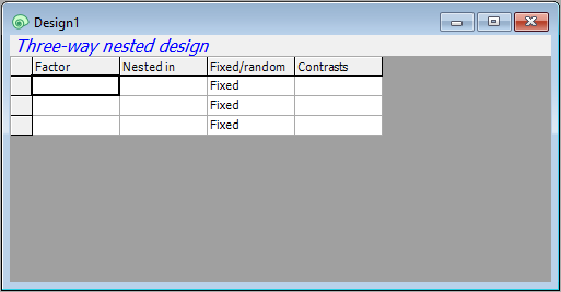
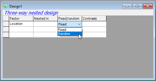
- Location: First, in row 1, click in the blank cell under the word 'Factor', and you will see a drop-down menu listing all of the factors associated with the resemblance matrix from which this design file was created. Choose 'Location' to fill this cell. Location is not nested in anything, so we leave the second cell in row 1 blank. In the third cell of row 1, we have to specify that Location is a random factor, so click on the word 'Fixed' and change it to 'Random'.
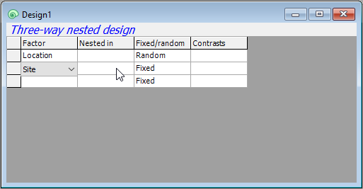
- Site: Next, we need to specify the second factor in the design in row 2 of the design file. Click on the cell in row 2 of the 'Factor' column (column 1) and choose 'Site'.
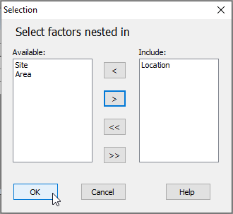
- Sites are nested in Locations, so we have to specify that in column two ('Nested in') accordingly. Click on the cell in row 2 in column 2 and a 'Selection' dialog will pop up to allow you to choose the factors within which 'Site' is nested. You will need to click on the word 'Location' (in the 'Available:' box on the left), then on the single-right-arrow button () to move it over into the 'Include:' box (on the right), then click OK, like so:
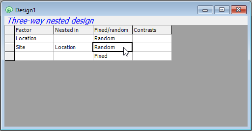
- Make sure that the factor 'Site' is also specified in column 3 as 'Random'. (This happens automatically after specifying a nested term in column 2, because nested terms are, almost always, random factors.) Your design file should now look like this:
- Area: Finally, we need to specify the third factor (Areas) correctly in row 3 of the design file. Under 'Factor' choose 'Area'. Under 'Nested in', specify 'Site', and make sure that column three has the word 'Random'. The final three-way nested design file should look like this:
Step 4: Run PERMANOVA
Once the design file is created, we are ready to go ahead with the PERMANOVA analysis.
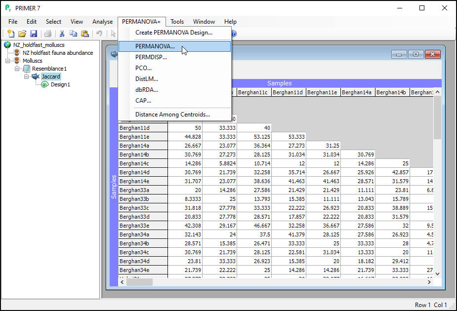
- Click on the 'Jaccard' resemblance matrix in the Explorer tree so that it is the active item in the workspace, then click PERMANOVA+ > PERMANOVA...
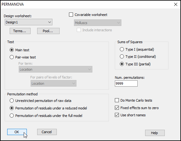
- Check to see that the 'Design worksheet:' is Design1; this is the design file we created in the previous step that contains the three-way nested design. For the rest, we will keep most of the defaults in the PERMANOVA dialog, but it is wise to increase 'Num. permutations:' from 999 to 9999, as shown below, then click OK.
- This produces an output file (called 'PERMANOVA1') in the Explorer tree. It shows:
- the details of the choices you made in the PERMANOVA dialog to run the analysis;
- the details of your experimental design; and
- the PERMANOVA table of results
as follows:
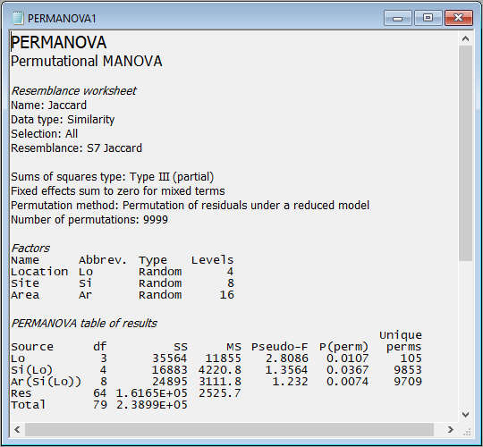
Interpretation
These results show that there is statistically significant variability in the identities of molluscs among holdfasts at each of the three spatial scales in the experimental design: Areas ($F_{8,64}$ = 1.23, $P$ < 0.01), Sites ($F_{4,8}$ = 1.36, $P$ < 0.05) and Locations ($F_{3,4}$ = 2.81, $P$ < 0.05). Note that the p-value for Locations is somewhat limited by the number of unique values of the pseudo-F statistic under permutation that are available here. Specifically, when we permute 2 samples per group (i.e., the 8 Sites) randomly across 4 groups (the Locations), there are just 105 unique values of pseudo-F that can be obtained, so the minimum possible p-value here is 1/105 = 0.0095).
Step 4 (continued): Key additional details about PERMANOVA in PRIMER
Following the PERMANOVA table of results, a suite of key additional details regarding the analysis can be seen in the PERMANOVA output file.
(Note: It is not necessary to fully unpack all of these details to continue on with the analysis and interpretation of results, but some information is provided here to highlight what makes the implementation of PERMANOVA in PRIMER so unique, surpassing all other software tools in its robust handling of multi-factorial experimental designs).
Additional details in the PERMANOVA output file include:
- details of the expected mean squares (EMS) for each term in the model;
- the construction of the pseudo-F ratios for each term in the model from the appropriate mean squares (along with the associated numerator and denominator degrees of freedom); and
- estimates of the components of variation for each term in the model in the space of the resemblance measure.
For example, scrolling down further in the output file from the PERMANOVA done on the holdfast data, we see:
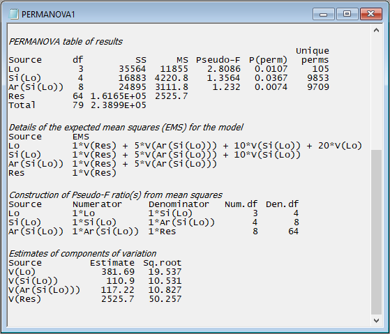
The implementation of PERMANOVA in PRIMER always uses expected mean squares (EMS) to construct correct tests for every term in the model; specifically:
- to construct the correct pseudo-F ratio; and
- to implement a permutation algorithm that
- identifies the correct permutable units; and
- accounts correctly for other terms in the model.
Of course, each term will require careful construction of its own test-statistic and its own permutation algorithm, both of which will depend on whether terms are fixed or random, whether there are other nested terms, covariates or interactions, etc. For unbalanced cases, the 'Type' of sum of squares is also important for the partitioning and correct construction of individual tests. All of these things can affect the EMS.
The EMS are also used to estimate the components of variation attributable to different sources of variation. These are not the same thing as raw $R^2$ values (as are typically used to compare the relative importance of individual predictor variables in regression models). In PERMANOVA, these are calculated in a directly analogous way to the unbiased univariate ANOVA estimators. The column labeled 'Estimate' expresses these components in squared dissimilarity units, and its square root ('Sq.root', interpretable as a sort of standard deviation in the space of the resemblance measure) is also provided.
In the present example, we can see that the greatest variation occurs at the smallest spatial scale - from holdfast to holdfast within a given area (i.e., the square root of 'V(Res)' is 50.257 in Jaccard % dissimilarity units). The sources of variation (in order of importance, as quantified by the PERMANOVA model) are: Residual > Location > Area > Site.
For more information about all of these key additional details provided in the PERMANOVA output file, please consult the PERMANOVA+ manual.
Step 5: Ordination of centroids
Having seen the results of a PERMANOVA analysis, it is natural to wish to see a visualisation of the patterns among centroids belonging to different groups or combinations of levels of different factors in the study design. In many cases, particularly if there is a large number of replicates in a complex study design, if one were simply to create an ordination of all individual sampling units, there would just be a lot of noise (the plot may look very messy), due to high residual variation. This tends to obscure salient patterns and important effects.
Ordination of sampling units (all replicates)
We can produce a non-metric MDS ordination of the holdfast data by starting from the Jaccard resemblance matrix and clicking on Analyse > MDS > Non-metric MDS..., taking all of the defaults, then clicking OK. The resulting configurations are very unsatisfactory with quite high stress, either in 2 dimensions (stress = 0.28, shown below), or 3 dimensions (stress = 0.20).
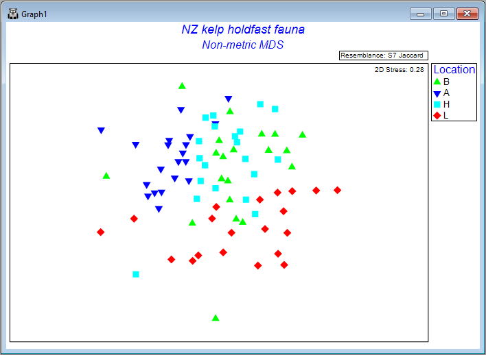
Seeing a bit of a 'mess' when we plot replicates like this is actually not too surprising in many cases, and particularly in this case, considering the very high variation (high turnover) in the identities of molluscs among holdfasts at small spatial scales (within areas), as seen on the previous page (recall that the residuals contributed by far the greatest source of variation to this system).
Ordination of distances among centroids
We can instead examine an ordination plot of the centroids in the space of the resemblance measure. In multi-factor designs when there is more than one factor and these factors are crossed with one another, we may need to created a single factor that consists of combinations of levels of the crossed factors (using Edit > Factors... > Combine...), but in the case of a fully nested design, and where nested factors all utilise unique labels (such as we have here), we can proceed without such a step.
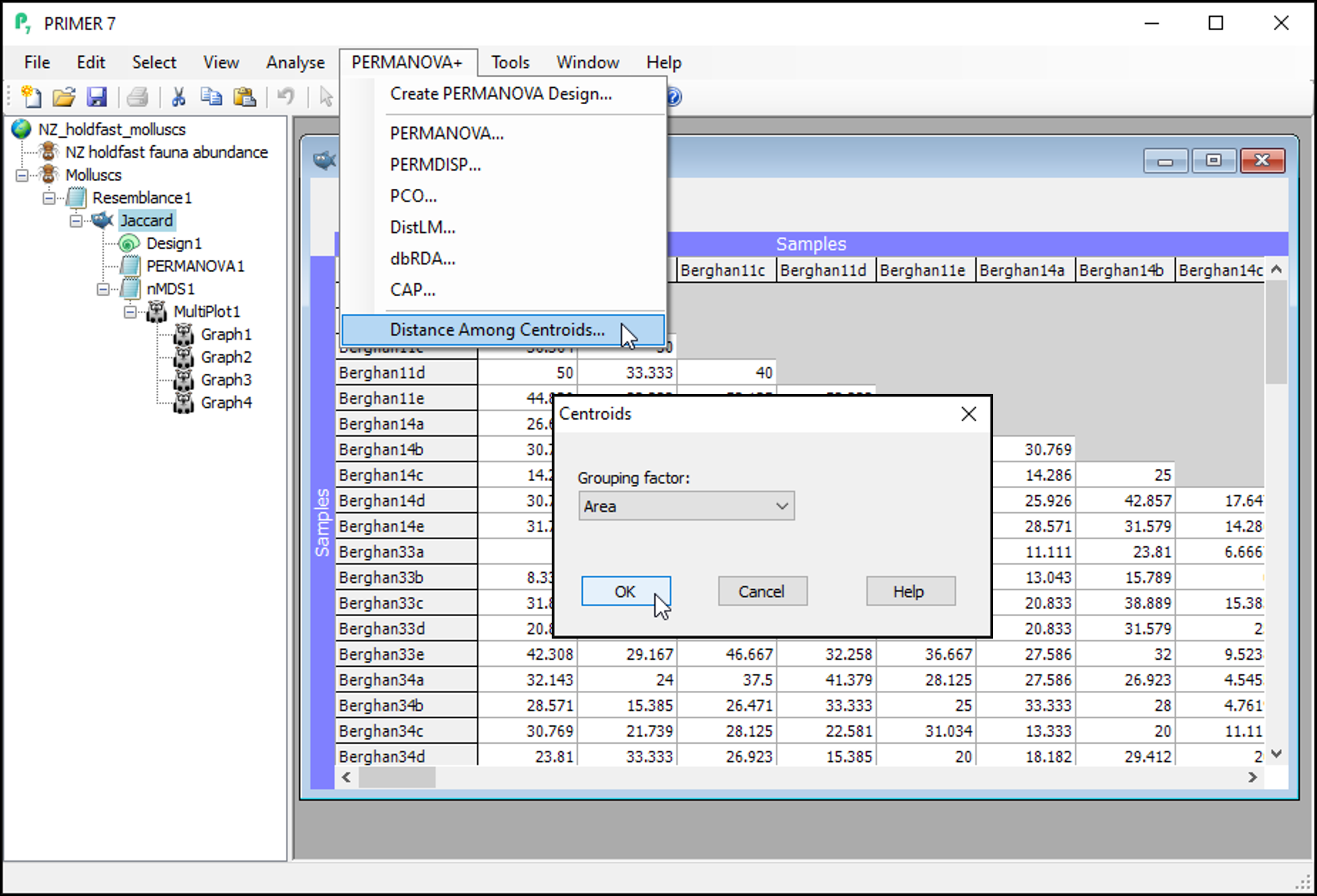
- From the 'Jaccard' resemblance matrix, click PERMANOVA+ > Distances Among Centroids, then in the 'Centroids' dialog, choose (Grouping factor: Area), and click OK.
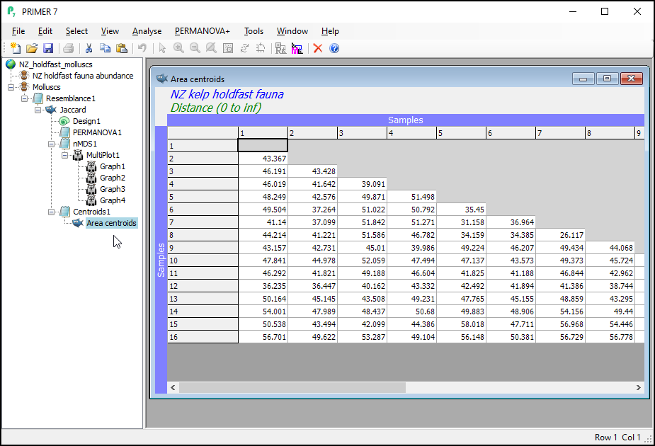
This will give you a matrix of Jaccard dissimilarities among the 16 Area centroids; each centroid being comprised of n = 5 replicate holdfasts within a given area. These are constructed in the space of the dissimilarity measure, which is not (quite) the same thing as calculating the arithmetic averages in the space of the original variables (i.e., that corresponds to a centroid in Euclidean space). In other words, these are the centroids just 'as PERMANOVA sees them' in Jaccard space, when doing the partitioning. You can re-name this matrix (from 'Resem1') to 'Area centroids'; i.e.,
-
From the 'Area centroids' resemblance matrix, click Analyse > MDS > Non-metric MDS..., take all the defaults and click OK.
-
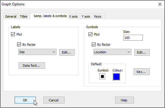
From the 2D nMDS (probably called 'Graph5'), click on Graph > Sample Labels & Symbols..., then choose (Labels > $\checkmark$Plot > $\checkmark$By factor > Site) & (Symbols > $\checkmark$Plot > $\checkmark$By factor > Location), then click OK.
The result is a much more interpretable ordination plot, with far lower stress, viz:
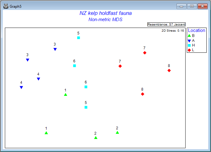
Each point now represents the centroid (in Jaccard space) for n = 5 holdfasts in a given area. The numbers identify the 8 different sites, and the colours correspond to the 4 different locations. The patterns we see here are consistent with what was learned from the PERMANOVA analysis. More specifically, we can see that, within any particular location, the variation from one area to the next (any 2 centroids having the same symbol and number) is fairly similar to the variation between the two sites (any 2 centroids having the same colour, but a different number), and also that variation among locations (different colours) exceeds this - all four locations are clearly distinguishable from one another on the plot.
Summary of the PERMANOVA analysis
A summary of the essential commands associated with performing this PERMANOVA analysis of the holdfast data according to the 3-factor hierarchical experimental design is given in the table below:
| Step | To implement in PRIMER: |
|---|---|
| 1. Select variable subset | From the original data sheet: click Select > Variables... > ($\bullet$Indicator levels > Indicator name: Phylum), click Levels...> (Selection > Include: Mollusca), click OK. |
| 2. Jaccard resemblance | From the subset-selected data sheet: click Analyse > Resemblance > (Measure $\bullet$Other > S7 Jaccard) & (Analyse between $\bullet$Samples), click OK. |
| 3. Specify the design |
|
| 4. Run PERMANOVA | From the resemblance matrix: click PERMANOVA+ > PERMANOVA... > (Design Worksheet: Design1) & (Num. permutations: 9999) & (default settings for the rest), click OK. |
| 5. Ordination of centroids |
|