Chapter 10: Species aggregation to higher taxa
10.1 Species aggregation
Fig. 10.1a repeats the multivariate ordination (nMDS) seen in Fig. 1.7 for the macrofaunal data from Frierfjord, based on 4th-root transformed species counts and Bray-Curtis similarities among the 24 samples (at 6 sites, A-E,G). The assemblage consisted of 110 taxa identified in three-quarters of the cases to the species level (the remainder, as is commonly the case, were only identified to some higher taxonomic level, e.g. Nemertines, Oligochaetes etc). Fig. 10.1b shows the same ordination plot that would have been obtained had all species-level identifications only been to the level of genus, and it is clear that the conclusions about the relationships among the 6 sites would have remained more or less identical had the identification level been that degree coarser. This is not really that surprising since many of the identified genera only contained a single species, the number of variables (taxa) reducing only from 110 species to 88 genera¶. However, the insensitivity of the multivariate analysis to the change in identification effort in this case is suggestive of more general possibilities.
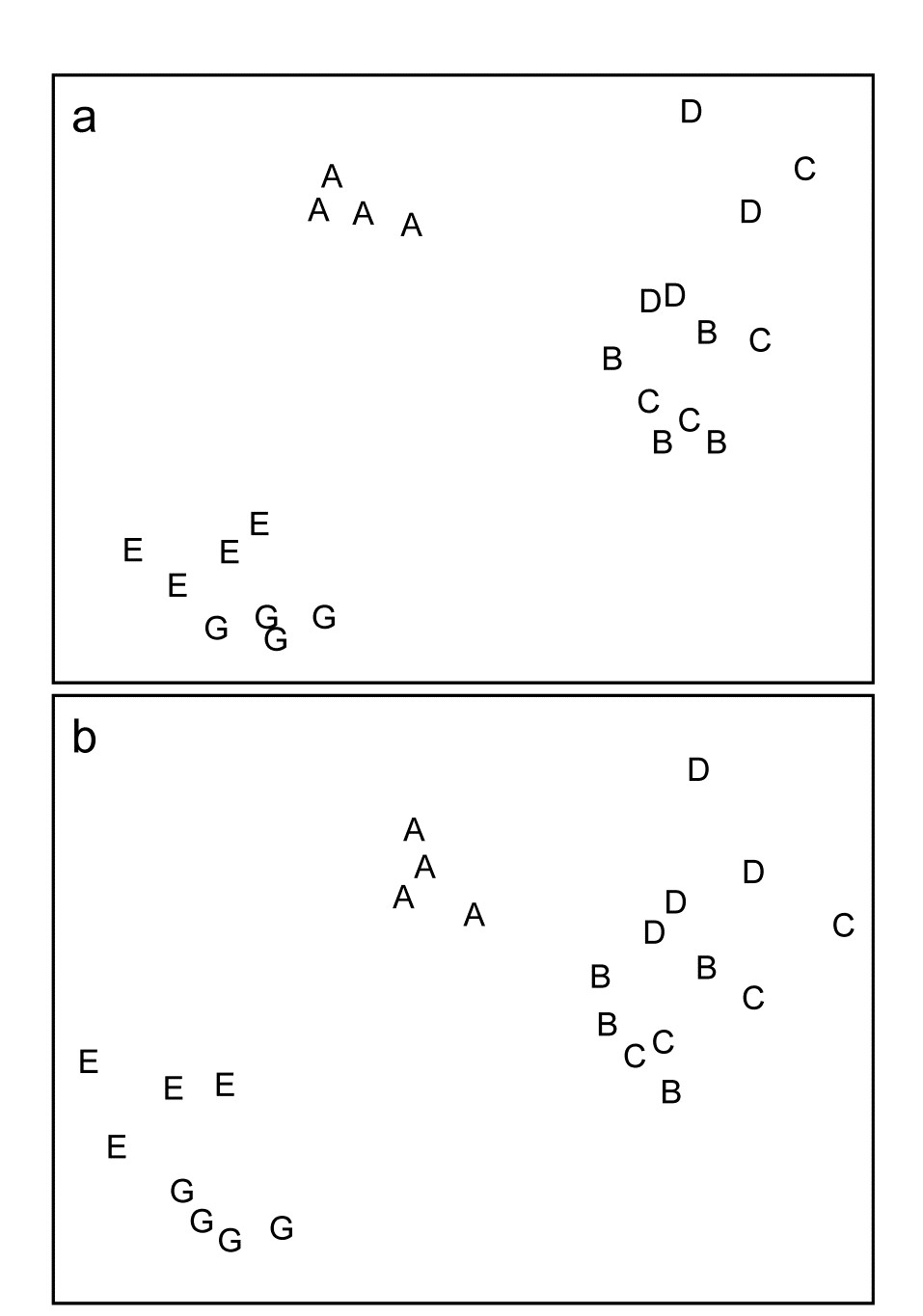
Fig. 10.1 Frierfjord macrofauna {F}. Sample MDS using Bray-Curtis similarities on $ \sqrt{} \sqrt{} $-transformed counts for a) 110 species, b) 88 genera (stress = 0.10, 0.09 respectively).
The painstaking work involved in sorting and identifying samples to the species level has resulted in community analysis for environmental impact studies being traditionally regarded as labour-intensive, time-consuming and therefore relatively expensive. One practical means of overcoming this problem might therefore be to try analysing the samples to some higher taxonomic level, such as family. If results from this coarser level are comparable to full species analysis, this means that:
a) A great deal of labour can be saved. Several groups of marine organisms are taxonomically difficult, for example (in the macrobenthos) several families of polychaetes and amphipods; as much time can be spent in separating a few of these difficult groups into species as the entire remainder of the sample, even in Northern Europe where taxonomic keys for identification are most readily available.
b) Less taxonomic expertise is needed. Many taxa really require the skills of specialists to separate them into species, and this is especially true in parts of the world where fauna is poorly described. For certain groups of marine organisms, e.g. the meiobenthos, the necessary expertise required to identify even the major taxa (nematodes and copepods) to species is lacking in most laboratories which are concerned with the monitoring of marine pollution, so that these components of the biota are rarely used in such studies, despite their many inherent advantages (see Chapter 13).
For the marine macro- and meiobenthos, aggregations of the species data to higher taxonomic levels are examined below in a few applications, and resultant data matrices subjected to several forms of statistical analysis to see how much information has been lost compared with species-level analysis. Examples are also seen in Chapter 16, where a more sophisticated methodology is given for summarising the relative effects of differing levels of taxonomic aggregation, in comparison with other decisions that need to be made about a multivariate analysis, e.g. severity of transformation and choice of resemblance measure (we defer such discussion until the needed tools have been presented in Chapters 11 and 15). Aggregation, followed by simple re-analysis, has now been looked at very widely in the marine (and non-marine) literature for a range of faunal groups.
Methods amenable to aggregation
- Multivariate methods. Although taxonomic levels higher than that of species can be used to some degree for all types of statistical analysis of community data, it is probably for multivariate methods that this is most appropriate, at least when the taxa is relatively species rich; e.g. Chapter 16 shows the high degree of structural redundancy in marine macrobenthic assemblages, with many sets of species ‘carrying the same information’, in effect, about the spatio-temporal changes which drive the community patterns. (On the other hand, it is clear that for a very limited faunal group such as, say, the freshwater fish of Australian river systems, with species numbers typically only in single figures, there is much to lose and little to gain by aggregation to higher taxa). All ordination/clustering techniques are amenable to aggregation, and there is now substantial evidence that identification only to the family level for macrobenthos, and the genus level for meiobenthos, makes very little difference to the results (see, for example, Figs. 10.2–10.6, and the results in Chapter 16). There are possibly also theoretical advantages to conducting multivariate analyses at a high taxonomic level for pollution impact studies. Natural environmental variables which also affect community structure are rarely constant in surveys designed to detect pollution effects over relatively large geographical areas. For the benthos, such ‘nuisance’ variables include water depth and sediment granulometry. However, it is a tenable hypothesis that these variables influence the fauna more by species replacement than by changes in the proportions of the major taxa present. Each major group, in its adaptive radiation, has evolved species which are suited to rather narrow ranges of natural environmental conditions, whereas anthropogenic contamination has been too recent for the evolution of suitably adapted species. Ordinations of abundance or biomass data of these major taxa are thus more likely to correlate with a contaminant gradient than are species ordinations, the latter being more complicated by the effects of natural environmental variables. In short, higher taxa may well reflect well-defined pollution gradients more closely than species.
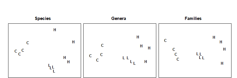
Fig. 10.2. Nutrient-enrichment experiment, Solbergstrand {N}. MDS plot of copepod abundances ($ \sqrt{} \sqrt{} $-transformed, Bray-Curtis similarities) for 4 replicates from 3 treatments; species data aggregated into genera and families (stress = 0.09, 0.09, 0.08).

Fig. 10.3. Loch Linnhe macrofauna {L}. MDS (using Bray-Curtis similarities) of samples from 11 years. Abundances are $ \sqrt{} \sqrt{} $-transformed (top) and untransformed (bottom), with 111 species (left), aggregated into 45 families (middle) and 9 phyla (right). (Reading across rows, stress = 0.09, 0.09, 0.10, 0.09, 0.09, 0.02).
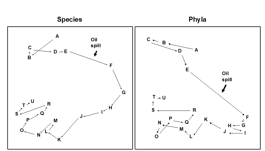
Fig. 10.4. Amoco-Cadiz oil spill {A}. MDS for macrobenthos at station ‘Pierre Noire’ in the Bay of Morlaix. Species data (left) aggregated into phyla (right). Sampling months are A:4/77, B:8/77, C:9/77, D:12/77, E:2/78, F:4/78, G:8/78, H:11/78, I:2/79, J:5/79, K:7/79, L:10/79, M:2/80, N:4/80, O:8/80, P:10/80, Q:1/81, R:4/81, S:8/81, T:11/81, U:2/82. The oil-spill was during 3/78, (stress = 0.09, 0.07).
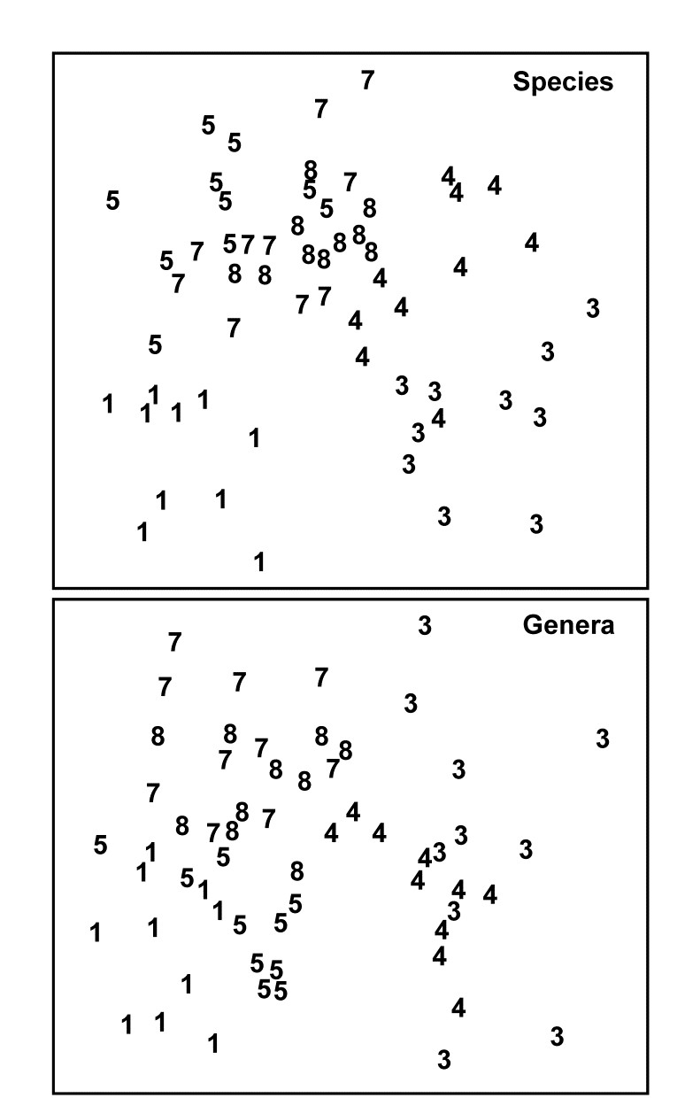
Fig. 10.5. Indonesian reef corals {I}. MDS for species (p=75) and genus (p=24) data at South Pari Island (Bray-Curtis similarities on untransformed % cover). The El Niño occurred in 1982–3. 1=1981, 3=1983 etc. (stress = 0.25).
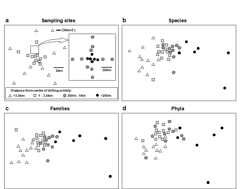
Fig. 10.6. Ekofisk oil-platform macrobenthos {E}. a) Map of station positions, indicating symbol/shading conventions for distance zones from the centre of drilling activity; b)-d) MDS for root-transformed species, family and phyla abundances (stress = 0.12, 0.11, 0.13).
-
Distributional methods. Aggregation for ABC curves is possible, and family level analyses are often identical to species level analyses (Fig. 10.7).
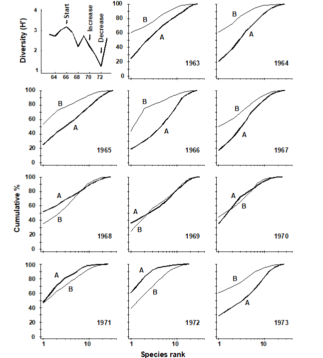
Fig. 10.7. Loch Linnhe macro¬fauna {L}. Shannon diversity (H´) and ABC plots over the 11 years, 1963 to 1973, for data aggregated to family level (c.f. Fig. 8.7). Abundance = thick line, biomass = thin line.
- Univariate methods. The concept of pollution indicator groups rather than indicator species is well-established. For example, at organically enriched sites, polychaetes of the family Capitellidae become abundant (not just Capitella capitata), as do meiobenthic nematodes of the family Oncholaimidae. The nematode copepod ratio ( Raffaelli & Mason (1981) ) is an example of a pollution index based on higher taxonomic levels. Such indices are likely to be of more general applicability than those based on species level data. Diversity indices themselves can be defined at hierarchical taxonomic levels for internal comparative purposes, although this is not commonly done in practice.
¶ This pooling of counts to any specified coarser taxonomic level (called aggregation by PRIMER) uses the Aggregate routine on the Tools menu and requires a look-up table, an aggregation file, which can consist of a much larger species set (probably in a different order), from which each variable (species) in the data matrix is allocated to a specified genus, family, order, class, etc. Such aggregation files are also of fundamental importance in computing biodiversity measures based on the taxonomic relatedness of species in each sample, see Chapter 17.
10.2 Examples
Multivariate examples
Nutrient-enrichment experiment
In the soft-bottom mesocosms at Solbergstrand, Norway {N}, box-cores of sublittoral sediment were subjected to three levels of particulate organic enrichment (L = low dose, H = high dose and C = control), there being four replicates from each treatment. After 56 days the meiobenthic communities were analysed. Fig 10.2 shows that, for the copepods, there were clear differences in community structure between treatments at the species level, which were equally evident when the species data were aggregated into genera and families. (Indeed, at the family level the configuration is arguably more linearly related to the pollution gradient than at the species level).
Loch Linnhe macrofauna
MDS ordinations of the Loch Linnhe macrobenthos are given in Fig. 10.3, using both double square root and untransformed abundance data. Information on the time-course of pollution events and changes in diversity are given in Fig. 10.7 (top left). The ordinations have been performed separately using all 111 species, the 45 families and the 9 phyla. In all ordinations there is a separation to the right of the years 1970, 1971 and 1972 associated with increasing pollution levels and community stress, and a return to the left in 1973 associated with reduced pollution levels and community stress. This pattern is equally clear at all levels of taxonomic aggregation. Again, the separation of the most polluted years is most distinct at the phylum level, at least for the double square root transformed data (and the configuration is more linear with respect to the pollution gradient at the phylum level for the untransformed data).
Amoco-Cadiz oil-spill
Macrofauna species were sampled at station ‘Pierre Noire’ in the Bay of Morlaix on 21 occasions between April 1977 and February 1982, spanning the period of the wreck of the ‘Amoco-Cadiz’ in March 1978. The sampling site was some 40km from the initial tanker disaster but substantial coastal oil slicks resulted. The species abundance MDS has been repeated with the data aggregated into five phyla: Annelida, Mollusca, Arthropoda, Echinodermata and ‘others’ (Fig. 10.4). The analysis of phyla closely reflects the timing of pollution events, the configuration being slightly more linear than in the species analysis. All pre-spill samples (A-E) are in the top left of the configuration, the immediate post-spill sample (F) shifts abruptly to the bottom right after which there is a gradual recovery in the pre-spill direction. Note that in the species analysis, although results are similar, the immediate post-spill response is rather more gradual. The community response at the phylum level is remarkably clear.
Indonesian reef corals
The El Niño of 1982-3 resulted in extensive bleaching of reef corals throughout the Pacific. Fig. 10.5 shows the coral community response at South Pari Island over six years in the period 1981-1988, based on ten replicate line transects along which coral species cover was determined. Note the immediate post-El Niño location shift on the species MDS and a circuitous return towards the pre-El Nino condition. This is closely reflected in the genus level analysis.
Ekofisk oil-platform macrobenthos
Changes in community structure of the soft-bottom benthic macrofauna in relation to oil drilling activity at the Ekofisk platform in the North Sea {E} have been studied by
Gray, Clarke, Warwick et al. (1990)
and
Warwick & Clarke (1991)
. The positions of the 39 sampling stations around the rig are coded by different symbol and shading conventions in Fig. 10.6a, according to their distance from the centre of drilling activity at that time. In the MDS species abundance analysis (Fig. 10.6b), community composition in all of the zones is distinct, and there is a clear gradation of change from the (black circle) inner to the (open triangle) outer zones. Formal significance testing (using the methods of Chapter 6) confirms statistically the differences between all zones. The MDS has been repeated with the species data aggregated into families (Fig. 10.6c) and phyla (Fig. 10.6d). The separation of sites is still clear, and pairwise comparisons confirm the statistical significance of differences between all zones, even at the phylum level, which does show some deterioration of the pattern. This is in contrast to (species-level) univariate and graphical/distributional measures, in which only the inner zone (less than 250m from the rig) was significantly different from the other three zones (see Chapter 14). Thus, phylum level analyses are again shown to be surprisingly sensitive in detecting pollution-induced community change, and little information at all is lost by working at the family level.
Graphical examples
Loch Linnhe macrofauna
ABC plots for the Loch Linnhe macrobenthos species data are given in Chapter 8, Fig. 8.7, where the performance of these curves with respect to the time-course of pollution events is discussed. In Fig. 10.7 the species data are aggregated to family level, and the curves are virtually identical to the species level analysis, so that there would have been no loss of information had the samples only been sorted originally into families.
Similar results were produced by replotting the ABC curves for the Garroch Head sewage sludge dumping ground macrobenthos {G} (Fig. 8.8) at the family level ( Warwick (1988b) ).
Univariate example
Indonesian reef corals
Fig. 10.8 shows results from another survey of 10 replicate line transects for coral cover over the period 1981-1988, in this case at South Tikus Island, Indonesia {I}. Note the similarity of the species and genus analyses for the number of taxa and Shannon diversity, with an immediate post-El Niño drop and subsequent suggestion of partial recovery.
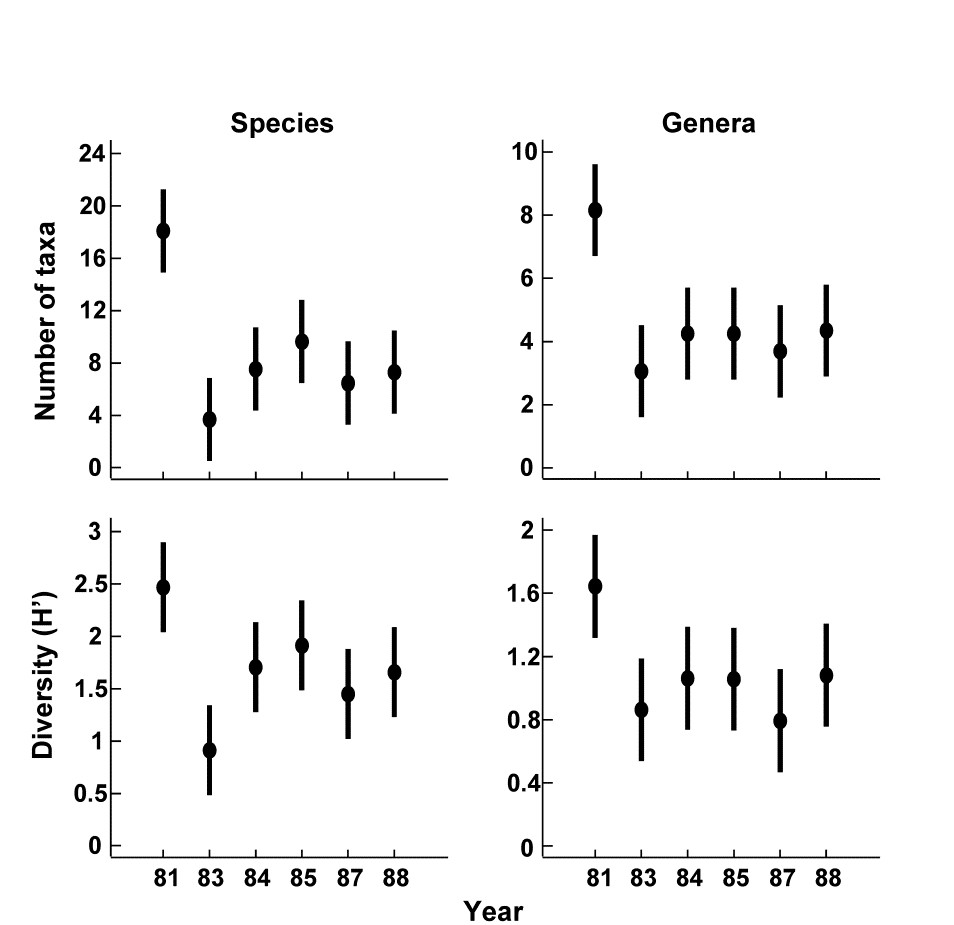
Fig. 10.8. Indonesian reef corals {I}. Means and 95% confidence intervals for number of taxa and Shannon diversity at South Tikus Island, showing the impact and partial recovery from the 1982–3 El Niño. Species data (left) have been aggregated into genera (right).
10.3 Recommendation
Clearly the operational taxonomic level for environmental impact studies is another factor to be considered when planning such a survey, along with decisions about the number of stations to be sampled, number of replicates, types of statistical analysis to be employed etc. The choice will depend on several factors, particularly the time, manpower and expertise available and the extent to which that component of the biota being studied is known to be robust to taxonomic aggregation, for the type of statistical analysis being employed, and the type of perturbation expected. Thus, it is difficult to give general recommendations and each case must be treated on its individual merits. However, for routine monitoring of organic enrichment situations using macrobenthos, one can by now be rather certain that family level analysis will be perfectly adequate. Also, for the free-living meiofauna, there are by now many examples where multivariate analysis of genus-level information is indistinguishable from that for species, and broadly similar results have been found now for a wide range of faunal groups. The topic is returned to in Chapter 16.