Chapter 12: Causality - community experiments in the field and laboratory
12.1 Introduction
In Chapter 11 we have seen how both the univariate and multivariate community attributes can be correlated with natural and anthropogenic environmental variables. With careful sampling design, these methods can provide strong evidence as to which environmental variables appear to affect community structure most, but they cannot actually prove cause and effect. In experimental situations we can investigate the effects of a single factor (the treatment) on community structure, while other factors are held constant or controlled, thus establishing cause and effect. There are three main study types which have been labelled ‘experiments’ (though many ecologists – and most statisticians! – would argue that it is a misnomer in the first case):
-
‘Natural experiments’. Nature provides the treatment, i.e. we compare places or times which differ in the intensity of the forcing factor in question.
-
Field experiments. The experimenter provides the treatment, i.e. environmental factors (biological, chemical or physical) are manipulated in the field.
- Laboratory experiments. Environmental factors are manipulated by the experimenter in laboratory mesocosms or microcosms.
The degree of ‘naturalness’ (hence realism) decreases from 1-3, but the degree of control which can be exerted over potentially confounding environmental variables increases from 1-3.
In this chapter, each class of experiments is illustrated by a single example. These all happen to concern the meiobenthos, since such data is readily available to the authors(!) but also because the smaller the biotic size component the more amenable it is to community level manipulations (see Chapter 13).
In all cases care should be taken to avoid pseudoreplication, i.e. the treatments should be replicated, rather than a series of (pseudo-)replicate samples taken from a single treatment (e.g. Hurlbert (1984) ). This is because other confounding variables, often unknown, may also differ between the treatments. It is also important to run experiments long enough for community changes to occur; this favours components of the fauna with short generation times (Chapter 13).
It should be made clear at the outset that the treatment of experiments in this chapter is somewhat cursory. The subject of ecological experiments requires a book of its own, indeed it gets an excellent one in Underwood (1997) . The latter, though, in common with other biologically oriented texts on experiments, concerns univariate analysis (e.g. of a population abundance). Ecological experiments with multiple outcomes using multivariate methods are now, however, commonplace in publications: useful methods papers include Anderson (2001a) ; Anderson (2001b) ; Chapman & Underwood (1999) ; Krzanowski (2002) ; Legendre & Anderson (1999) ; McArdle & Anderson (2001) ; Underwood & Chapman (1998) ; Clarke, Somerfield, Airoldi et al. (2006) .
¶ A self-evident truth from the explosion of assemblage studies using the PRIMER and PERMANOVA+ multivariate methods on microbiological communities in the last few years, many of which are a result of manipulative experiments. This manual is deficient in not representing such studies in its illustrations, but it is clear that there are few, if any, different issues of principle in carrying over the macro-scale examples to microbiological or genetic contexts.
12.2 `Natural experiments’
It is doubtful whether so called natural experiments deserve to be called ‘experiments’ at all, and not simply well-designed field surveys, since they make comparisons of places or times which differ in the intensity of the particular environmental factor under consideration. The obvious logical flaw with this approach is that its validity rests on the assumption that places or times differ only in the intensity of the selected environmental factor (treatment); there is no possibility of randomly allocating treatments to experimental units, the central tool of experimentation and one that ensures that the potential effects of unmeasured, uncontrolled variables are averaged out across the experimental groups. Design is often a problem, but statistical techniques such as two-way ANOVA, e.g. Sokal & Rohlf (1981) , Underwood (1981) , or two-way ANOSIM (Chapter 6), may enable us to examine the treatment effect allowing for differences between sites, for example. This is illustrated in the first example below.
In some cases natural experiments may be the only possible approach for hypothesis testing in community ecology, because the attribute of community structure under consideration may result from evolutionary rather than ecological mechanisms, and we obviously cannot conduct manipulative field or laboratory experiments over evolutionary time. One example of a community attribute which may be determined by evolutionary mechanisms relates to size spectra in marine benthic communities. Several hypotheses, some complementary and some contradictory, have been invoked to explain biomass size spectra and species size distributions in the metazoan benthos, both of which have bimodal patterns in shallow temperate shelf seas. Ecological explanations involve physical constraints of the sedimentary environment, animals needing to be small enough to move between the particles (i.e. interstitial) or big enough to burrow, with an intermediate size range capable of neither ( Schwinghamer (1981) ). Evolutionary explanations invoke the optimisation of two size-related sets of reproductive and feeding traits: for example small animals (meiobenthos) have direct benthic development and can be dispersed as adults, large animals (macrobenthos) have planktonic larval development and dispersal, there being no room for compromise ( Warwick (1984) ).
To test these hypotheses we can compare situations where the causal mechanisms differ and therefore give rise to different predictions about pattern. For example, the reproductive dichotomy noted above between macrobenthos and meiobenthos breaks down in the deep-sea, in polar latitudes and in fresh water, although the physical sediment constraints in these situations will be the same as in temperate shelf seas. The evolutionary hypothesis therefore predicts that there should be a unimodal pattern in these situations, whereas the ecological hypothesis predicts that it should remain bimodal. Using these situations as natural experiments, we can therefore falsify one or the other (or both) of these hypotheses.
However, natural experiments of this kind are outwith this manual’s scope, and the chosen example concerns ecological effects of disturbance on assemblages.
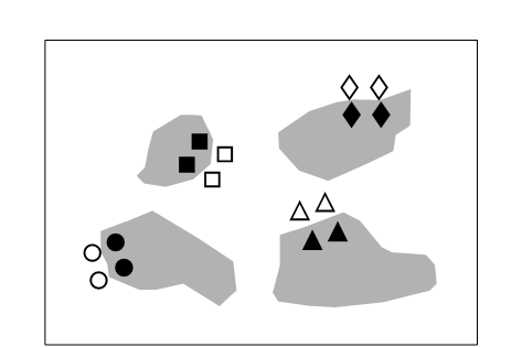
Fig. 12.1. Tasmania, Eaglehawk Neck {T}. Sketch showing the type of sample design. Sample positions (same symbols as in Fig. 12.3) in relation to disturbed sediment patches (shaded).
The effects of disturbance by soldier crabs on meiobenthic community structure {T}
On a sheltered intertidal sandflat at Eaglehawk Neck, on the Tasman Peninsula in S.E. Tasmania, the burrowing and feeding activities of the soldier crab Mictyris platycheles are evidenced as intensely disturbed areas of sediment which form discrete patches interspersed with smooth undisturbed areas. The crabs feed by manipulating sand grains in their mandibles and removing fine particulate material, but they are not predators on the meiofauna, though their feeding and burrowing activity results in intense sediment disturbance. This situation was used as a ‘natural experiment’ on the effects of disturbance on meiobenthic community structure. Meiofauna samples were collected in a spatially blocked design, such that each block comprised two disturbed and two undisturbed samples, each 5m apart (Fig. 12.1).
Table 12.1. Tasmania, Eaglehawk Neck {T}. Mean values per core sample of univariate measures for nematodes, copepods and total meiofauna (nematodes + copepods) in the disturbed and undisturbed areas. The significance levels for differences are from a two-way ANOVA, i.e. they allow for differences between blocks, although these were not significant at the 5% level.
Total individuals (N) |
Total species (S) |
Species richness (d) |
Shannon diversity (H’) |
Species evenness (J’) |
|
|---|---|---|---|---|---|
| Nematodes | |||||
| Disturbed | 205 | 14.4 | 2.6 | 1.6 | 0.58 |
Undisturbed |
200 | 20.1 | 3.7 | 2.2 | 0.74 |
| Significance (%) | 91 |
1 |
0.3 | 0.1 | 1 |
| Copepods | |||||
| Disturbed | 94 |
5.4 | 1.0 | 0.96 | 0.59 |
| Undisturbed | 146 | 5.7 |
1.0 | 0.84 | 0.49 |
| Significance (%) | 11 |
52 |
99 | 52 |
38 |
| Disturbed | 299 | 19.8 | 3.4 | 2.0 | 0.66 |
| Undisturbed | 346 | 25.9 | 4.4 | 2.3 | 0.69 |
| Significance (%) | 48 |
1 |
3 |
3 |
16 |

Univariate indices. The significance of differences between disturbed and undisturbed samples (treatments) was tested with two-way ANOVA (blocks/treatments), Table 12.1. For the nematodes, species richness, Shannon diversity and evenness were significantly reduced in disturbed as opposed to undisturbed areas, although total abundance was unaffected. For the copepods, however, there were no significant differences in any of these univariate measures.
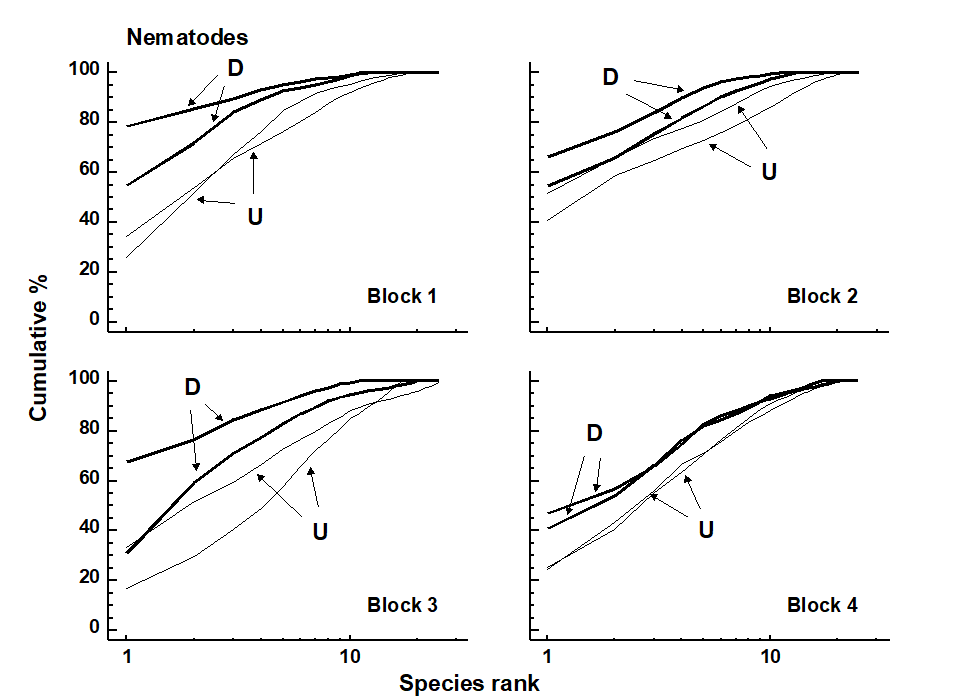
Fig. 12.2. Tasmania, Eaglehawk Neck {T}. Replicate k-dominance curves for nematode abundance in each sampling block. D = disturbed, U = undisturbed.
Graphical/distributional plots. k-dominance curves (Fig. 12.2) also revealed significant differences in the relative species abundance distributions for nematodes (using both ANOVA and ANOSIM-based tests, the latter following DOMDIS, as described on page 8.5, see
Clarke (1990)
). For the copepods, however, (plots given in Chapter 13, Fig. 13.4), k-dominance curves are intermingled and crossing, and there is no significant treatment effect.
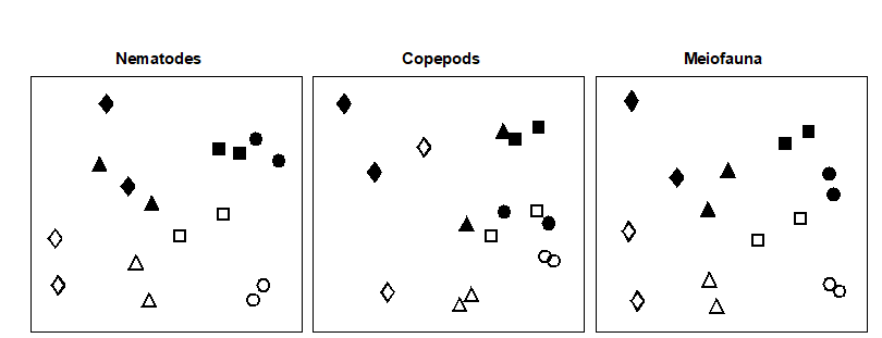
Fig. 12.3. Tasmania, Eaglehawk Neck {T}. MDS configurations for nematode, copepod and ‘meiofauna’ (nematode + copepod) abundance (root-transformed). Different shapes represent the four blocks of samples. Open symbols = undisturbed, filled = disturbed (stress = 0.12, 0.09. 0.11 respectively).
Table 12.2. Tasmania, Eaglehawk Neck {T}. Results of the two-way ANOSIM test for treatment (disturbance/no disturbance) and block effects.
| Disturbance |  Blocks Blocks |
||||
|---|---|---|---|---|---|
| R | Sig.(%) | R | Sig.(%) | ||
| Nematodes | 1.0 | 1.2 | 0.85 | 0.0 | |
| Copepods | 0.56 | 3.7 | 0.62 | 0.0 | |
| Meiofauna | 0.94 | 1.2 | 0.85 | 0.0 |
Multivariate ordinations. MDS revealed significant differences in species composition for both nematodes and copepods: the effects of crab disturbance were similar within each block and similar for nematodes and copepods. Though the ‘treatment signal’ is weaker for the latter, note the general similarities in Fig. 12.3 between the nematode and copepod configurations: both disturbed samples within each block are above both of the undisturbed samples (except for one block for the copepods), and the blocks are arranged in the same sequence across the plot. For both nematodes and copepods, two-way ANOSIM shows a significant effect of both treatment (disturbance) and blocks, Table 12.2, but the differences are more marked for the nematodes (with higher values of the R statistic).
Conclusions. Univariate indices and graphical/distributional plots were only significantly affected by crab disturbance for the nematodes. Multivariate analysis revealed a similar response for nematodes and copepods (i.e. it seems to be a more sensitive measure of community change). In multivariate analyses, natural variations in species composition across the beach (i.e. between blocks) were about as great as those between treatments within blocks, and the disturbance effect would not have been clearly evidenced without this blocked sampling design.
12.3 Field experiments
Field manipulative experiments include, for example, caging experiments to exclude or include predators, controlled pollution of experimental plots, and big-bag experiments with plankton. Their use was historically (unsurprisingly) predominantly for univariate population rather than community studies, although some early examples of multivariate analysis of manipulative field experiments include Anderson & Underwood (1997) , Morrisey, Underwood & Howitt (1996) , Gee & Somerfield (1997) and Austen & Thrush (2001) . The following example is one in which univariate, graphical and multivariate statistical analyses have been applied to meiobenthic communities.
Azoic sediment recolonisation experiment with predator exclusion {Z}
Olafsson & Moore (1992) studied meiofaunal colonisation of azoic sediment in a variety of cages designed to exclude epibenthic macrofauna to varying degrees: A – 1 mm mesh cages designed to exclude all macrofauna; B –1 mm control cages with two ends left open; C – 10 mm mesh cages to exclude only larger macro-fauna; D – 10 mm control cages with two ends left open; E – open unmeshed cages; F – uncaged background controls. Three replicates of each treatment were sampled after 1 month, 3 months and 8 months and analysed for nematode and harpacticoid copepod species composition.
Univariate indices. The presence of cages had a more pronounced impact on copepod diversity than nematode diversity. For example, after 8 months, $H ^ \prime$ and $J ^ \prime$ (but not $S$) for copepods had significantly higher values inside the exclusion cages than in the control cages with the ends left open, but for the nematodes, differences in $H ^ \prime$ were of borderline significance (p = 5.3%).
Graphical/distributional plots. No significant treatment effect for either nematodes or copepods could be detected between k-dominance curves for all sampling dates, using the ANOSIM test for curves, referred towards the end of Chapter 8 (page 8.5).
Multivariate analysis. For the harpacticoid copepods there was a clear successional pattern of change in community composition over time (Fig. 12.4), but no such pattern was obvious for the nematodes. Fig. 12.4 uses data from Table 2 in Olafsson and Moore’s paper, which are for the 15 most abundant harpacticoid species in all treatments and for the mean abundances of all replicates within a treatment on each sampling date. On the basis of these data, there is no significant treatment effect using the 2-way crossed ANOSIM test with no replication¶ (see page 6.8), but the fuller replicated data may have been more revealing.
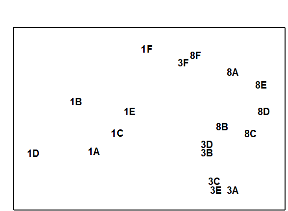
Fig. 12.4. Azoic sediment recolonisation experiment {Z}. MDS configuration for harpacticoid copepods (4th root transformed abundances) after 1, 3 and 8 months, with 6 different treatments (A–F), see text (stress = 0.07).
¶ Note, however, that this test (or the equivalent PERMANOVA test which exploits the interaction term as its residual) will be uninformative in the presence of large treatment $\times$ time interactions, which is a likely possibility here.
12.4 Laboratory experiments
More or less natural communities of some components of the biota can be maintained in laboratory (and also outdoor) experimental containers and subjected to a variety of manipulations. Many types of experimental systems have been used for marine studies, ranging from microcosms (containers less than 1 m$^3$) to mesocosms (1–1000 m$^3$). Early examples of microcosm experiments analysed by multivariate means can be found, for example, in
Austen & McEvoy (1997)
,
Schratzberger & Warwick (1998b)
,
Schratzberger & Warwick (1999)
, and mesocosm experiments in
Austen, Widdicombe & Villano-Pitacco (1998)
,
Widdicombe & Austen (1998)
and
Widdicombe & Austen (2001)
. Macrocosms (larger than $10 ^ 3$ m$^ 3$), usually involving the artificial enclosure of natural areas in the field, have also been used, for pelagic studies, though replicating the treatment is often a significant problem.
Effects of organic enrichment on meiofaunal community structure {N}
Gee, Warwick, Schaanning et al. (1985)
collected undisturbed box cores of sublittoral sediment and transferred them to the experimental mesocosms established at Solbergstrand, Oslofjord, Norway. They produced organic enrichment by the addition of powdered Ascophyllum nodosum to the surface of the cores, in quantities equivalent to 50 g C m$^{-2}$ (four replicate boxes) and 200 g C m$^{-2}$ (four replicate boxes), with four undosed boxes as controls, in a randomised design within one of the large mesocosm basins. After 56 days, five small core samples of sediment were taken from each box and combined to give one sample. The structure of the meiofaunal communities in these samples was then compared.
Univariate indices. Table12.3 shows that, for the nematodes, there were no significant differences in species richness or Shannon diversity between treatments, but evenness was significantly higher in enriched boxes than controls. For the copepods, there were significant differences in species richness and evenness between treatments, but not in Shannon diversity.
Table 12.3. Nutrient-enrichment experiment {N}. Univariate measures for all replicates at the end of the experiment, with the F-ratio and significance levels from one-way ANOVA.
Species richness (d) |
Shannon diversity (H') |
Species evenness (J') |
|
|---|---|---|---|
| Nematodes | |||
| Control | 3.02 | 2.25 | 0.750 |
| 3.74 | 2.39 | 0.774 | |
| 3.36 | 2.47 | 0.824 | |
| 4.59 | 2.76 | 0.747 | |
| Low dose | 4.39 | 2.86 | 0.877 |
| 2.65 | 2.47 | 0.840 | |
| 4.67 | 2.89 | 0.875 | |
| 2.33 | 2.27 | 0.860 | |
| High dose | 2.86 | 2.17 | 0.782 |
| 2.82 | 2.39 | 0.843 | |
| 4.30 | 2.40 | 0.829 | |
| 4.09 | 2.47 | 0.853 | |
| F ratio | 0.04 | 1.39 | 5.13 |
| Sig level (p) | ns | ns | <5% |
| Copepods | |||
| Control | 2.53 | 1.93 | 0.927 |
| 1.92 | 1.56 | 0.969 | |
| 2.50 | 1.77 | 0.908 | |
| 2.47 | 1.94 | 0.931 | |
| Low dose | 1.80 | 1.60 | 0.643 |
| 1.66 | 1.28 | 0.532 | |
| 1.66 | 1.16 | 0.484 | |
| 1.79 | 1.54 | 0.640 | |
| High dose | 1.75 | 1.59 | 0.767 |
| 0.97 | 1.00 | 0.620 | |
| 1.03 | 0.30 | 0.165 | |
| 1.18 | 1.70 | 0.872 | |
| F ratio | 17.72 | 2.65 | 4.56 |
| Sig level (p) | <0.1% | ns | <5% |
Graphical/distributional plots. Fig. 12.5 shows the average k-dominance curves over all four boxes in each treatment. For the nematodes these are closely coincident, suggesting no obvious treatment effect. For the copepods, however, there are apparent differences between the curves. A notable feature of the copepod assemblages in the enriched boxes was the presence, in highly variable numbers, of several species of the large epibenthic harpacticoid Tisbe, which are ‘weed’ species often found in old aquaria and associated with organic enrichment. If this genus is omitted from the analysis, a clear sequence of increasing elevation of the k-dominance curves is evident from control to high dose boxes.

Fig. 12.5. Nutrient enrichment experiment {N}. k-dominance curves for nematodes, total copepods and copepods omitting the ‘weed’ species of Tisbe, for summed replicates of each treatment, C = control, L = low and H = high dose.
Table 12.4. Nutrient enrichment experiment {N}. Values of the R statistic from the ANOSIM test, in pairwise comparisons between treatments, together with significance levels. C = control, L = low dose, H = high dose.
| Treatment | Statistic value (R) |
% Sig. level |
|
|---|---|---|---|
| Nematodes | |||
| (L,C) | 0.27 | 2.9 | |
| (H,C) | 0.22 | 5.7 | |
| (H,L) | 0.28 | 8.6 | |
| Copepods | |||
| (L,C) | 1.00 | 2.9 | |
| (H,C) | 0.97 | 2.9 | |
| (H,L) | 0.59 | 2.9 |
Multivariate analysis. Fig. 12.6 shows that, in an MDS of $\sqrt{} \sqrt{}$-transformed species abundance data, there is no obvious discrimination between treatments for the nematodes. In the ANOSIM test (Table 12.4) the values of the R statistic in pairwise comparisons between treatments are low (0.2–0.3), but there is a significant difference between the low dose treatment and the control, at the 5% level. For the copepods, there is a clear separation of treatments on the MDS, the R statistic values are much higher (0.6–1.0), and there are significant differences in community structure between all treatments.
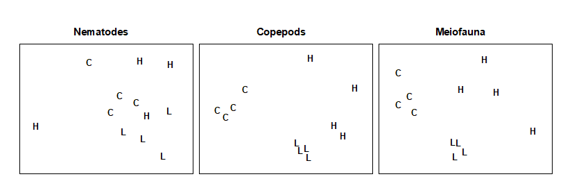
Fig. 12.6. Nutrient enrichment experiment {N}. MDS of $\sqrt{} \sqrt{}$-transformed abundances of nematodes, copepods and total meiofauna (nematodes + copepods). C = control, L = low dose, H = high dose (stress = 0.18, 0.09, 0.12).
Conclusions. The univariate and graphical/distributional techniques show lowered diversity with increasing dose for copepods, but no effect on nematodes. The multivariate techniques clearly discriminate between treatments for copepods, and still have some discriminating power for nematodes. Clearly the copepods have been much more strongly affected by the treatments in all these analyses, but changes in the nematode community may not have been detectable because of the great variability in abundance of nematodes in the high dose boxes. The responses observed in the mesocosm were similar to those sometimes observed in the field where organic enrichment occurs. For example, there was an increase in abundance of epibenthic copepods (particularly Tisbe spp.) resulting in a decrease in the nematode/copepod ratio. In this experiment, however, the causal link is closer to being established, though the possible constraints and artefacts inherent in any laboratory mesocosm study should always be borne in mind (see, for example, the discussion in Underwood & Peterson (1988) ).