Chapter 14: Relative sensitivities and merits of univariate, graphical/distributional and multivariate techniques

• 14.1 Introduction
• 14.2 Examples 1, 2 and 3
• 14.3 Examples 4, 5, 6 and 7
• 14.4 General conclusions and recommendations

14.1 Introduction

Two communities with a completely different taxonomic composition may have identical univariate or graphical/ distributional structure, and conversely those comprising the same species may have very different univariate or graphical structure. This chapter compares univariate, graphical and multivariate methods of data analysis by applying them to a broad range of studies on various components of the marine biota from a variety of localities, in order to address the question of whether species dependent and species independent attributes of community structure behave the same or differently in response to environmental changes, and which are the most sensitive. Within each class of methods we have seen in previous chapters that there is a very wide variety of different techniques employed, and to make this comparative exercise more tractable we have chosen to examine only one method for each class:

• Shannon-Wiener diversity index $H ^ \prime$ (see Chapter 8),

• k-dominance curves including ABC plots (Chapter 8),

• non-metric MDS ordination on a Bray-Curtis similarity matrix of appropriately transformed species abundance or biomass data (Chapter 5).

14.2 Examples 1, 2 and 3

Example 1: Macrobenthos from Frierfjord/Langesundfjord, Norway

As part of the GEEP/IOC Oslo Workshop, macrobenthos samples were collected at a series of six stations in Frierfjord/Langesundfjord {F}, station A being the outermost and station G the innermost (station F was not sampled for macrobenthos). For a map of the sampling locations see Fig. 1.1.

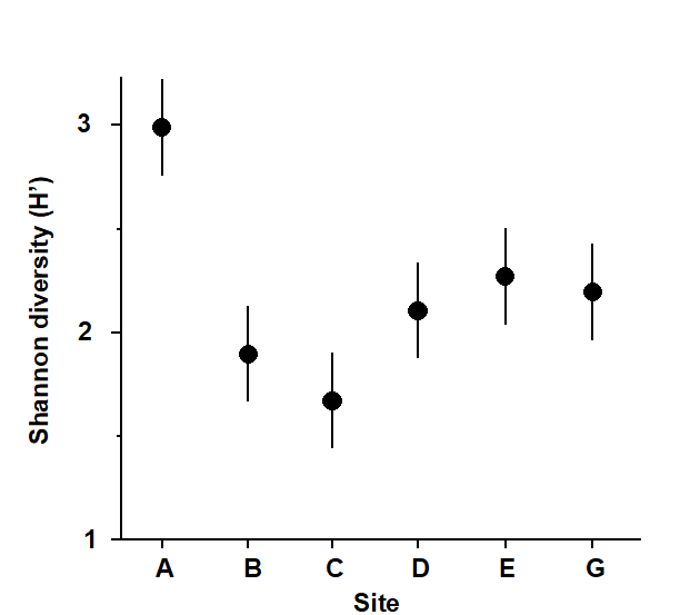
Fig. 14.1. Frierfjord macrobenthos {F}. Shannon diversity (mean and 95% confidence intervals) for each station.
 

Univariate indices

Site A had a higher species diversity and site C the lowest but the others were not significantly different (Fig. 14.1).
 

Graphical/distributional plots

ABC plots indicated that stations C, D and E were most stressed, B was moderately stressed, and A and G were unstressed (Fig. 14.2).

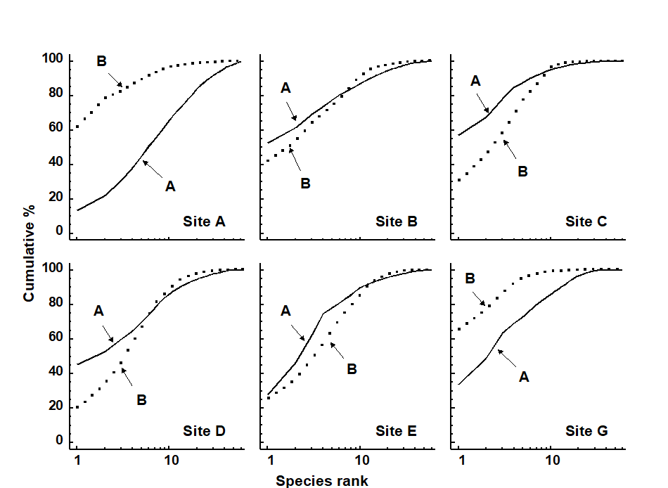
Fig. 14.2. Frierfjord macrobenthos {F}. ABC plots based on the totals from 4 replicates at each of the 6 sites. Solid lines: abundances; dotted lines: biomass.
 

Multivariate analysis

An MDS of all 24 samples (4 replicates at each station), supported by the ANOSIM test, showed that only stations B and C were not significantly different from each other (Fig. 14.3). Gray, Aschan, Carr et al. (1988) show that the clusters correlate with water depth rather than with measured levels of anthropogenic variables such as hydrocarbons or metals.

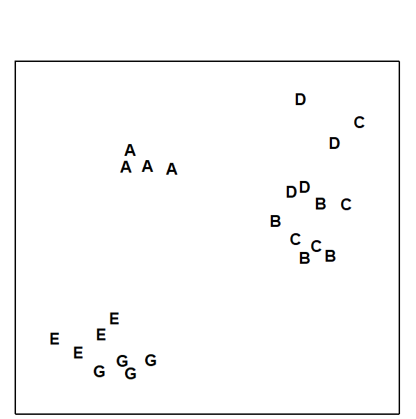
Fig. 14.3. Frierfjord macrobenthos {F}. MDS of 4 replicates at each of sites A–E, G, from Bray-Curtis similarities on 4th root-transformed counts (stress = 0.10).
 

Conclusions

The MDS was much better at discriminating between stations than the diversity measure, but perhaps more importantly, sites with similar univariate or graphical/ distributional community structure did not cluster together on the MDS. For example, diversity at E was not significantly different from D but they are furthest apart on the MDS; conversely, E and G had different ABC plots but clustered together. However, B, C and D all have low diversity and the ABC plots indicate disturbance at these stations. The most likely explanation is that these deep-water stations are affected by seasonal anoxia, rather than anthropogenic pollution.
 
 

Example 2: Macrobenthos from the Ekofisk oilfield, N. Sea

Changes in community structure of the soft-bottom benthic macrofauna in relation to oil drilling activity at the Ekofisk platform in the North Sea {E} have been described by Gray, Clarke, Warwick et al. (1990) . The positions of the sampling stations around the rig are coded by shading and symbol conventions in Fig. 14.4a, according to their distance from the active centre of drilling activity at the time of sampling.

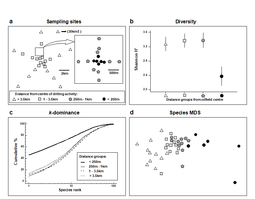
Fig. 14.4. Ekofisk macrobenthos {E}. a) Map of sampling sites, represented by different symbol and shading conventions according to their distance from the 2/4K rig at the centre of drilling activity; b) Shannon diversity (mean and 95% confidence intervals) in these distance zones; c) mean k-dominance curves; d) MDS from root-transformed species abundances (stress = 0.12).
 

Univariate indices

It can be seen from Fig. 14.4b that species diversity was only significantly reduced in the zone closer than 250m from the rig, and that the three outer zones did not differ from each other in terms of Shannon diversity (this conclusion extends to the other standard measures such as species richness and other evenness indices).
 

Graphical/distributional plots

The k-dominance curves (Fig. 14.4c) also only indicate a significant effect within the inner zone, the curves for the three outer zones being closely coincident.
 

Multivariate analysis

In the MDS analysis (Fig. 14.4d) community composition in all of the zones was distinct, and there was a clear gradation of change from the inner to outer zones. Formal significance testing (using ANOSIM) confirmed statistically the differences between all zones. It will be recalled from Chapter 10 that there was also a clear distinction between all zones at higher taxonomic levels than species (e.g. family), even at the phylum level for some zones.
 

Conclusions

Univariate and graphical methods of data analysis suggest that the effects on the benthic fauna are rather localised. The MDS is clearly more sensitive, and can detect differences in community structure up to 3 km away from the centre of activity.
 

Example 3: Reef corals at South Pari Island, Indonesia

Warwick, Clarke & Suharsono (1990) analysed coral community responses to the El Niño of 1982-3 at two reef sites in the Thousand Islands, Indonesia {I}, based on 10 replicate line transects for each of the years 1981, 83, 84, 85, 87 and 88.
 

Univariate indices

At Pari Island there was an immediate reduction in diversity in 1983, apparent full recovery by 1985, with a subsequent but not significant reduction (Fig. 14.5).

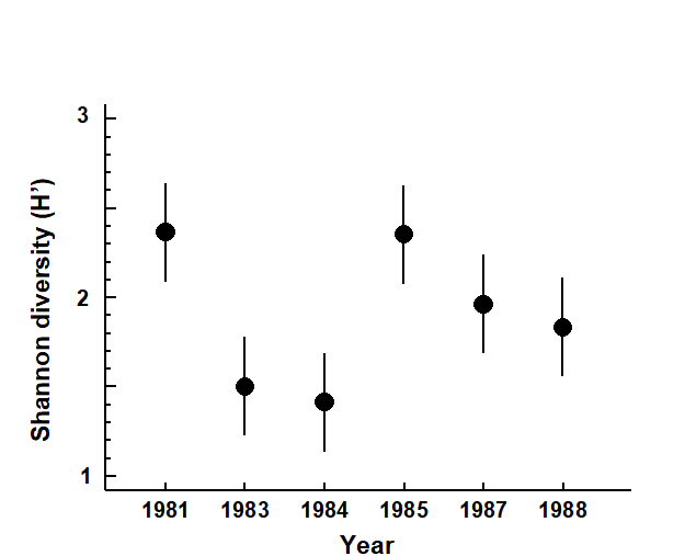
Fig. 14.5. Indonesian reef corals, Pari Island {I}. Shannon diversity (means and 95% confidence intervals) of the species coral cover from 10 transects in each year.
 

Graphical/distributional plots

The mean k-dominance curves were similar in 1981 and 1985, with the curves for 1983, 1984, 1987 and 1988 more elevated (Fig. 14.6). Tests on the replicate curves (using the DOMDIS routine given on page 8.5, followed by ANOSIM) confirmed the significance of differences between 1981, 1985 and the other years, but the latter were not distinguishable from each other.

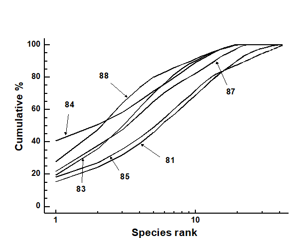
Fig. 14.6. Indonesian reef-corals, Pari Island {I}. k-dominance curves for totals of all ten replicates in each year.
 

Multivariate analysis

Though the MDS has rather a high stress it nonetheless shows an immediate location shift in community composition at the ten replicate sites between 1981 and 1983, and ANOSIM indicates significant differences between all pairs of years. Recovery proceeded in the pre-El Niño direction but was not complete by 1988 (Fig. 14.7).

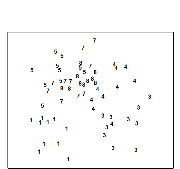
Fig. 14.7. Indonesian reef-corals, Pari Island {I}. MDS for coral species percentage cover data (1 = 1981, 3 = 1983 etc).
 

Conclusions

All methods of data analysis demonstrated the dramatic post El Niño decline in species, though the multivariate techniques were seen to be more sensitive in monitoring the recovery phase in later years.

14.3 Examples 4, 5, 6 and 7

Example 4: Fish communities from coral reefs in the Maldives

In the Maldive islands, Dawson-Shepherd, Warwick, Clarke et al. (1992) compared reef-fish assemblages at 23 coral reef-flat sites {M}, 11 of which had been subjected to coral mining for the construction industry and 12 were non-mined controls. The reef-slopes adjacent to these flats were also surveyed.
 

Univariate indices

Using ANOVA, no significant differences in diversity (Fig. 14.8) were observed between mined and control sites, with no differences either between reef flats and slopes.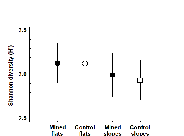

Fig. 14.8. Maldive Islands, coral-reef fish {M}. Shannon species diversity (means and 95% confidence intervals) at mined (closed symbols) and control (open symbols) sites, for both reef flats (circles) and reef slopes (squares).
 

Graphical/distributional plots

No significant differences could be detected between mined and control sites, in k-dominance curves for either species abundance or biomass. Fig. 14.9 displays the mean curves for reef-flat data pooled across the replicates for each condition.

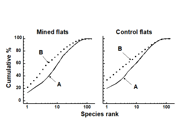
Fig. 14.9. Maldive Islands, coral-reef fish {M}. Average k-dominance curves for abundance and biomass at mined and control reef-flat sites.
 

Multivariate analysis

The MDS (Fig.14.10) clearly distinguished mined from control sites on the reef-flats, and also to a lesser degree even on the slopes adjacent to these flats, where ANOSIM confirmed the significance of this difference.

Fig. 14.10. Maldive Islands, coral-reef fish {M}. MDS of 4th root-transformed species abundance data. Symbols as in Fig. 14.8, i.e. circles = reef-flat, squares = slope, solid = mined, open = control (stress = 0.09).
 

Conclusions

There were clear differences in community composition due to mining activity revealed by multivariate methods, even on the reef-slopes adjacent to the mined flats, but these were not detected at all by univariate or graphical/ distributional techniques, even on the flats, where the separation in the MDS is so obvious.
 

Example 5: Macro- and meiobenthos from Isles of Scilly seaweeds

The entire metazoan fauna (macrofauna + meiofauna) has been analysed from five species of intertidal macro-algae (Chondrus, Laurencia, Lomentaria, Cladophora, Polysiphonia) each collected at eight sites near low water from rocky shores on the Isles of Scilly {S} (Fig. 14.11).

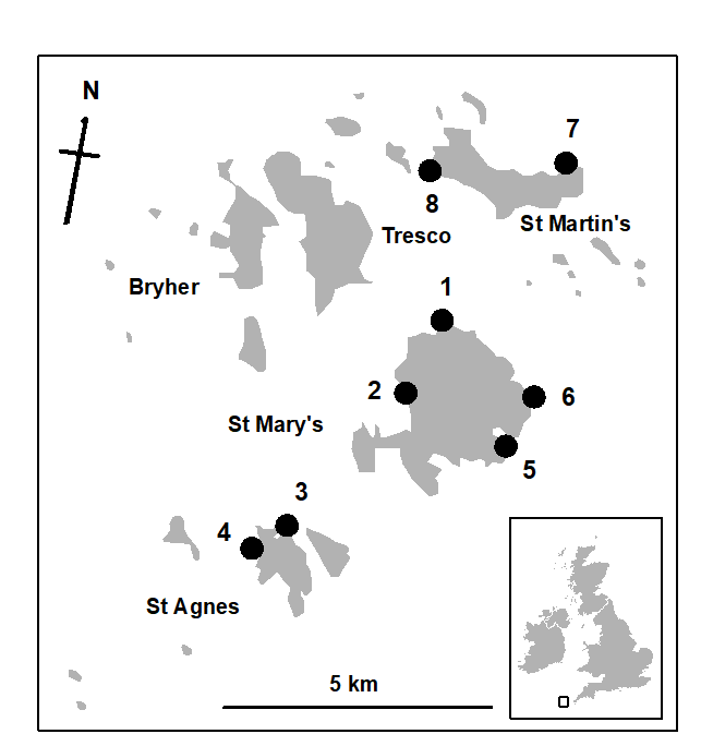
Fig. 14.11. Scilly Isles {S}. Map of the sites (1-8) from each of which 5 seaweed species were collected.
 

Univariate indices

The meiofauna and macrofauna showed clearly different diversity patterns with respect to weed type; for the meiofauna there was a trend of increasing diversity from the coarsest (Chondrus) to the finest (Polysiphonia) weed, but for the macrofauna there was no clear trend and Polysiphonia had the lowest diversity (Fig. 14.12).

Fig. 14.12. Isles of Scilly seaweed fauna {S}. Shannon diversity (mean and 95% confidence intervals) for the meiofauna and macrofauna of different weed species: Ch = Chondrus, La = Laurencia, Lo = Lomentaria, Cl = Cladophora, Po = Polysiphonia.
 

Graphical/distributional plots

These differences in meiofauna and macrofauna species diversity profiles were also reflected in the k-dominance curves (Fig. 14.13) which had different sequencing for these two faunal components, for example the Polysiphonia curve was the lowest for meiofauna and highest for macrofauna.

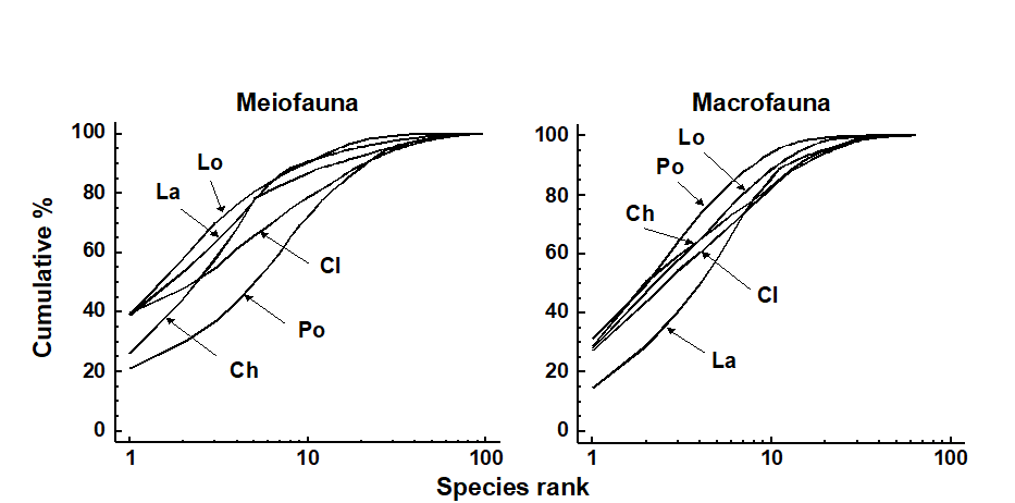
Fig. 14.13. Isles of Scilly seaweed fauna {S}. k-dominance curves for meiofauna (left) and macrofauna (right). Ch = Chondrus, La = Laurencia, Lo = Lomentaria, Cl = Cladophora, Po = Polysiphonia.
 

Multivariate analysis

The MDS plots for meiobenthos and macrobenthos were very similar, with the algal species showing very similar relationships to each other in terms of their meiofaunal and macrofaunal community structure (see Fig. 13.7, in which the shading and symbol conventions for the different weed species are the same as those in Fig. 14.12). Two-way crossed ANOSIM (factors: weed species and site), using the form without replicates (page 6.8), showed all weed species to be significantly different from each other in the composition of both macrofauna and meiofauna.
 

Conclusions

The MDS was more sensitive than the univariate or graphical methods for discriminating between weed species. Univariate and graphical methods gave different results for macrobenthos and meiobenthos, whereas for the multivariate methods the results were similar for both.
   

Example 6: Meiobenthos from the Tamar Estuary, S.W. England

Austen & Warwick (1989) compared the structure of the two major taxonomic components of the meiobenthos, nematodes and harpacticoid copepods, in the Tamar estuary {R}. Six replicate samples were taken at a series of ten intertidal soft-sediment sites (Fig. 14.14).

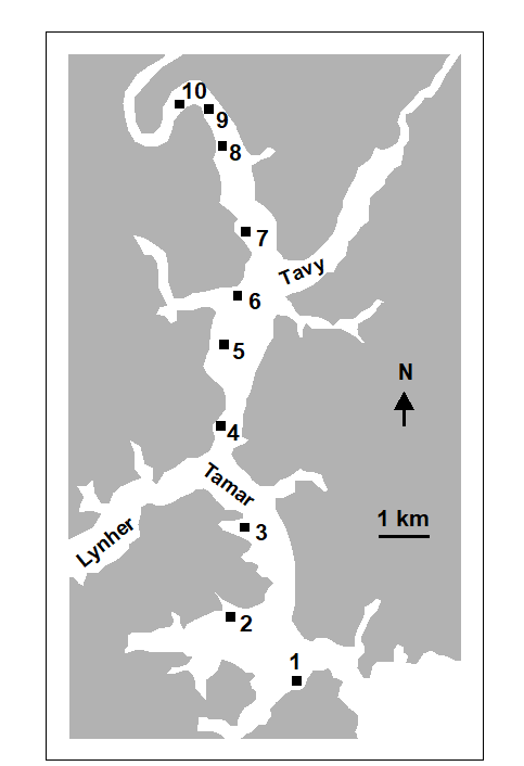
Fig. 14.14. Tamar estuary meiobenthos {R}. Map showing locations of 10 intertidal mud-flat sites.
 

Graphical/distributional plots

The average k-dominance curves showed no clear sequencing of sites for the nematodes, for example the curve for site 1 was closely coincident with that for site 10 (Fig. 14.15). For the copepods, however, the curves became increasingly elevated from the mouth to the head of the estuary. However, for both nematodes and copepods, many of the curves were not distinguishable from each other.

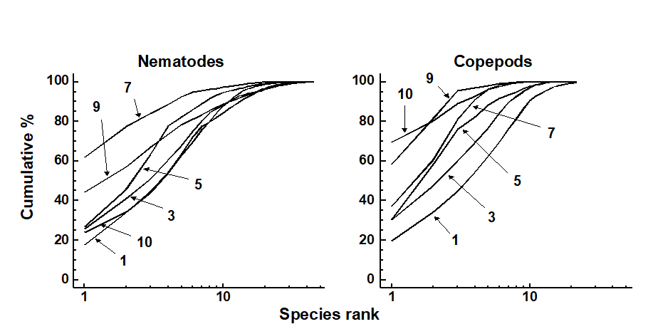
Fig. 14.15. Tamar estuary meiobenthos {R}. k-dominance curves for amalgamated data from 6 replicate cores for nematode and copepod species abundances. For clarity of presentation, some sites have been omitted.
 

Multivariate analysis

In the MDS, both nematodes and copepods showed a similar (arched) sequencing of sites from the mouth to the head of the estuary (Fig. 14.16). ANOSIM showed that the copepod assemblages were significantly different in all pairs of sites, and the nematodes in all pairs except 6/7 and 8/9.

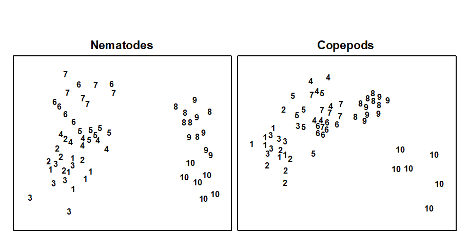
Fig. 14.16. Tamar estuary meiobenthos {R}. MDS of 4th root-transformed nematode and copepod species abundance data for six replicate cores at each of 10 stations.
 

Conclusions

The multivariate technique was more sensitive in discriminating between sites, and gave similar patterns for nematodes and copepods, whereas graphical methods gave different patterns for the two taxa. For nematodes, factors other than salinity seemed to be more important in determining diversity profiles, but for copepods salinity correlated well with diversity.
 

Example 7: Meiofauna from Eaglehawk Neck sandflat, Tasmania

This example of the effect of disturbance by burrowing and feeding of soldier crabs {T} was dealt with in some detail in Chapter 12. For nematodes, univariate, graphical and multivariate methods all distinguished disturbed from undisturbed sites. For copepods only the multivariate methods did. Univariate and graphical methods indicated different responses for nematodes and copepods, whereas the multivariate methods indicated a similar response for these two taxa.

14.4 General conclusions and recommendations

General conclusions

Three general conclusions emerge from these examples:

1. The similarity in community structure between sites or times based on their univariate or graphical/distributional attributes is different from their clustering in the multivariate analysis.
    

2. The species-dependent multivariate method is much more sensitive than the species-independent methods in discriminating between sites or times.
    

3. In examples where more than one component of the fauna has been studied, univariate and graphical methods may give different results for different components, whereas multivariate methods tend to give the same results.

The sensitive multivariate methods are essentially geared towards detecting differences in community composition between sites. Although these differences can be correlated with measured levels of stressors such as pollutants, the multivariate methods so far described do not in themselves indicate deleterious change which can be used in value judgements. Only the species-independent methods of data analysis lend themselves to the determination of deleterious responses although, as we have seen in Chapter 8 (and will do so again in Chapter 17), even the interpretation of changes in diversity is not always straightforward in these terms. There is a need to employ sensitive techniques for determining stress which utilise the full multivariate information contained in a species/sites matrix, and three such possibilities form the subject of the next chapter.
 

Recommendations

It is important to apply a wide variety of classes of data analysis, as each will give different information and this will aid interpretation. Sensitive multivariate methods will give an ‘early warning’ that community changes are occurring, but indications that these changes are deleterious are required by environmental managers, and the less sensitive taxa-independent methods will also play a role. Amongst the latter are the newly-devised biodiversity measures based on taxonomic (or phylogenetic) distinctness of the species making up a sample – see the discussion in Chapter 17 of their advantages over classical diversity indices.