Chapter 15: Multivariate measures of community stress and relating to models
- 15.1 Introduction
- 15.2 Meta-analysis of marine macrobenthos
- 15.3 Increased variability
- 15.4 Breakdown of seriation
- 15.5 Model matrices & ‘RELATE’ tests
- 15.6 Examples
15.1 Introduction
We have seen in Chapter 14 that multivariate methods of analysis are very sensitive for detecting differences in community structure between samples in space, or changes over time. Generally, however, these methods are used to detect differences between communities, and not in themselves as measures of community stress in the same sense that species-independent methods (e.g. diversity, ABC curves) are employed. Even using the relatively less-sensitive species-independent methods there may be problems of interpretation in this context. Diversity does not behave consistently or predictably in response to environmental stress. Both theory ( Connell (1978) ; Huston (1979) ) and empirical observation (e.g. Dauvin (1984) ; Widdicombe & Austen (1998) ) suggest that increasing levels of disturbance may either decrease or increase diversity, or it may even remain the same. A monotonic response would be easier to interpret. False indications of disturbance using the ABC method may also arise when, as sometimes happens, the species responsible for elevated abundance curves are pollution sensitive rather than pollution tolerant species (e.g. small amphipods, Hydrobia etc). Knowledge of the actual identities of the species involved will therefore aid the interpretation of ABC curves, and the resulting conclusions will be derived from an informal hybrid of species-independent and species-dependent information ( Warwick & Clarke (1994) ). In this chapter we describe three possible approaches to the measurement of community stress using the fully species-dependent multivariate methods.
15.2 Meta-analysis of marine macrobenthos
This method was initially devised as a means of comparing the severity of community stress between various cases of both anthropogenic and natural disturbance. On initial consideration, measures of community degradation which are independent of the taxonomic identity of the species involved would be most appropriate for such comparative studies. Species composition varies so much from place to place depending on local environmental conditions that any general species-dependent response to stress would be masked by this variability. However, diversity measures are also sensitive to changes in natural environmental variables and an unperturbed community in one locality could easily have the same diversity as a perturbed community in another. Also, to obtain comparative data on species diversity requires a highly skilled and painstaking analysis of species and a high degree of standardisation with respect to the degree of taxonomic rigour applied to the sample analysis; e.g. it is not valid to compare diversity at one site where one taxon is designated as Nematodes with another at which this taxon has been divided into species.
The problem of natural variability in species composition from place to place can be potentially overcome by working at taxonomic levels higher than species. The taxonomic composition of natural communities tends to become increasingly similar at these higher levels. Although two communities may have no species in common, they will almost certainly comprise the same phyla. For soft-bottom marine benthos, we have already seen in Chapter 10 that disturbance effects are detectable with multivariate methods often at the highest taxonomic levels, even in some instances where these effects are rather subtle and are not evidenced in univariate measures even at the species level, e.g. the Ekofisk {E} study.
Meta-analysis is a term widely used in biomedical statistics and refers to the combined analysis of a range of individual case-studies which in themselves are of limited value but in combination provide a more global insight into the problem under investigation. Warwick & Clarke (1993a) have combined macrobenthic data aggregated to phyla from a range of case studies {J} relating to varying types of disturbance, and also from sites which are regarded as unaffected by such perturbations. A choice was made of the most ecologically meaningful units in which to work, bearing in mind the fact that abundance is a rather poor measure of such relevance, biomass is better and production is perhaps the most relevant of all (Chapter 13). Of course, no studies have measured production (P) of all species within a community, but many studies provide both abundance (A) and biomass (B) data. Production was therefore approximated using the allometric equation:
$$ P = (B/A) ^ {0.73} \times A \tag{15.1} $$
where B/A is simply the mean body-weight, and 0.73 is the average exponent of the regression of annual production on body-size for macrobenthic invertebrates. Since the data from each study are standardised (i.e. production of each phylum is expressed as a proportion of the total) the intercept of this regression is irrelevant. For each data set the abundance and biomass data were first aggregated to phyla, following the classification of Howson (1987) ; 14 phyla were encountered overall (see the later Table 15.1). Abundance and biomass were then combined to form a production matrix using the above formula. All data sets were then merged into a single production matrix and an MDS performed on the standardised, 4th root-transformed data using the Bray-Curtis similarity measure. All macrobenthic studies from a single region (the NE Atlantic shelf) for which both abundance and biomass data were available were used, as follows:
-
A transect of 12 stations sampled in 1983 on a west-east transect (Fig. 1.5) across a sewage sludge dump-ground at Garroch Head, Firth of Clyde, Scotland {G}. Stations in the middle of the transect show clear signs of gross pollution.
-
A time series of samples from 1963–1973 at two stations (sites 34 and 2, Fig. 1.3) in West Scottish sea-lochs, L. Linnhe and L. Eil {L}, covering the period of commissioning of a pulp-mill. The later years show increasing pollution effects on the macrofauna, except that in 1973 a recovery was noted in L. Linnhe following a decrease in pollution loading.
-
Samples collected at six stations in Frierfjord (Oslofjord), Norway {F}. The stations (Fig. 1.1) were ranked in order of increasing stress A–G–E–D–B–C, based on thirteen different criteria. The macrofauna at stations B, C and D were considered to be influenced by seasonal anoxia in the deeper basins of the fjord.
-
Amoco-Cadiz oil spill, Bay of Morlaix {A}. In order not to swamp the analysis with one study, the 21 sampling times have been aggregated into 5 years for the meta-analysis: 1977 = pre-spill year, 1978 = post-spill year and 1979-81 = ‘recovery’ period.
-
Two stations in the Skagerrak at depths of 100 and 300m. The 300m station showed signs of disturbance attributable to the dominance of the sediment reworking bivalve Abra nitida.
-
An undisturbed station off the coast of Northumberland, NE England.
-
An undisturbed station in Carmarthen Bay, S Wales.
-
An undisturbed station in Kiel Bay; mean of 22 sets of samples.
In all, this gave a total of 50 samples, the disturbance status of which has been assessed by a variety of different methods including univariate indices, dominance plots, ABC curves, measured contaminant levels etc. The MDS for all samples (Fig.15.1) takes the form of a wedge with the pointed end to the right and the wide end to the left. It is immediately apparent that the long axis of the configuration represents a scale of disturbance, with the most disturbed samples to the right and the undisturbed samples to the left. (The reason for the spread of sites on the vertical axis is less obvious). The relative positions of samples on the horizontal axis can thus be used as a measure of the relative severity of disturbance. Another gratifying feature of this plot is that in all cases increasing levels of disturbance result in a shift in the same direction, i.e. to the right. For visual clarity, the samples from individual case studies are plotted in Fig. 15.2, with the remaining samples represented as dots.
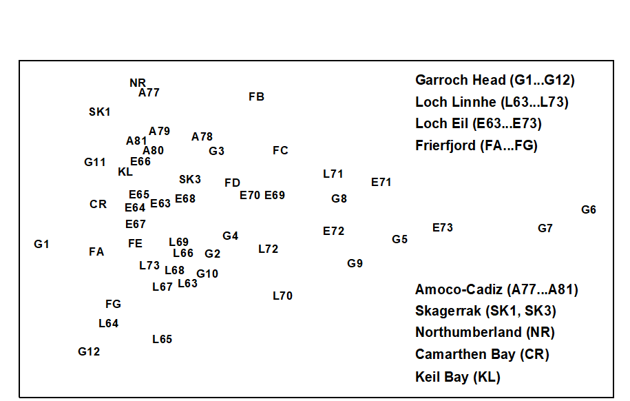
Fig. 15.1. Joint NE Atlantic shelf studies (‘meta-analysis’) {J}. Two dimensional MDS ordination of phylum level ‘production’ data (stress = 0.16).
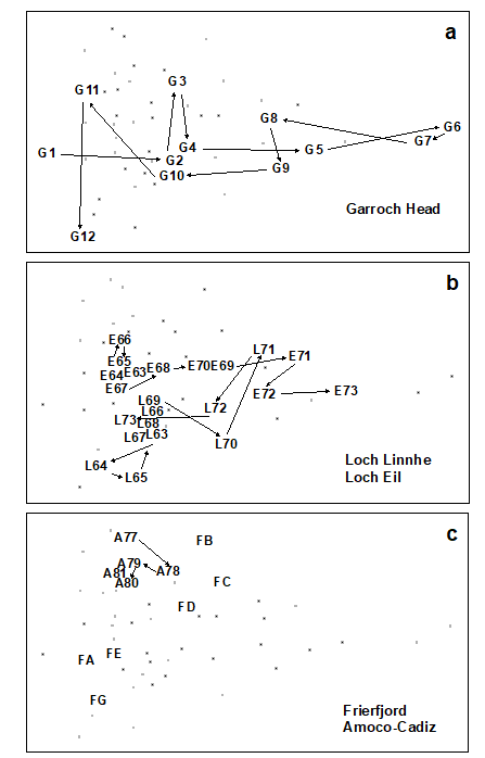
Fig. 15.2. Joint NE Atlantic shelf studies (‘meta-analysis’) {J}. As Fig. 15.1 but with individual studies highlighted: a) Garroch Head (Clyde) dump-ground; b) Loch Linnhe and Loch Eil; c) Frierfjord and Amoco-Cadiz spill (Morlaix).
-
Garroch Head (Clyde) sludge dump-ground {G}. Samples taken along this transect span the full scale of the long axis of the configuration (Fig. 15.2a). Stations at the two extremities of the transect (1 and 12) are at the extreme left of the wedge, and stations close to the dump centre (6) are at the extreme right.
-
Loch Linnhe and Loch Eil {L}. In the early years (1963–68) both stations are situated at the unpolluted left-hand end of the configuration (Fig. 15.2b). After this the L. Eil station moves towards the right, and at the end of the sampling period (1973) it is close to the right-hand end; only the sites at the centre of the Clyde dump-site are more polluted. The L. Linnhe station is rather less affected and the previously mentioned recovery in 1973 is evidenced by the return to the left-hand end of the wedge.
-
Frierfjord (Oslofjord) {F}. The left to right order of stations in the meta-analysis is A–G–E–D–B–C (Fig. 15.2c), exactly matching the ranking in order of increasing stress. Note that the three stations affected by seasonal anoxia (B,C and D) are well to the right of the other three, but are not as severely disturbed as the organically enriched sites in 1) and 2) above.
-
Amoco-Cadiz spill, Morlaix {A}. Note the shift to the right between 1977 (pre-spill) and 1978 (post-spill), and the subsequent return to the left in 1979–81 (Fig. 15.2c). However, the shift is relatively small, suggesting that this is only a mild effect.
-
Skagerrak. The biologically disturbed 300m station is well to the right of the undisturbed 100m station, although the former is still quite close to the left-hand end of the wedge.
-
to 8 Unpolluted sites. The Northumberland, Carmarthen Bay and Keil Bay stations are all situated at the left-hand end of the wedge.
An initial premise of this method was that, at the phylum level, the taxonomic composition of communities is relatively less affected by natural environmental variables than by pollution or disturbance (Chapter 10). To examine this, Warwick & Clarke (1993a) superimposed symbols scaled in size according to the values of the two most important environmental variables considered to influence community structure, sediment grain size and water depth, onto the meta-analysis MDS configuration (a technique described in Chapter 11). Both variables had high and low values scattered arbitrarily across the configuration, which supports the original assumption.
With respect to individual phyla, annelids comprise a high proportion of the total ‘production’ at the polluted end of the wedge, with a decrease at the least polluted sites. Molluscs are also present at all sites, except the two most polluted, and have increasingly higher dominance towards the non-polluted end of the wedge. Echinoderms are even more concentrated at the non-polluted end, with some tendency for higher dominance at the bottom of the configuration (Fig. 15.3a). Crustacea are again concentrated to the left, but this time entirely confined to the top part of the configuration (Fig. 15.3b). Clearly, the differences in relative proportions of crustaceans and echinoderms are largely responsible for the vertical spread of samples at this end of the wedge, but these differences cannot be explained in terms of the effects of any recorded natural environmental variables. Nematoda are clearly more important at the polluted end of the wedge, an obvious consequence of the fact that species associated with organic enrichment tend to be very large in comparison with their normal meiofaunal counterparts (e.g. Oncholaimids), and are therefore retained on the macrofaunal ecologists’ sieves. Other less important phyla show no clear distribution pattern, except that most are absent from the extreme right-hand samples.
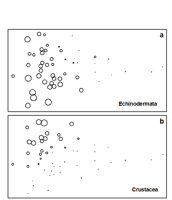
Fig. 15.3. Joint NE Atlantic shelf studies (‘meta-analysis’) {J}. As Fig. 15.1 but highlighting the role of specific phyla in shaping the MDS; symbol size represents % production in each sample from: a) echinoderms, b) crustaceans.
This multivariate approach to the comparative scaling of benthic community responses to environmental stress seems to be more satisfactory than taxon-independent methods, having both generality and consistency of behaviour. It is difficult to assess the sensitivity of the technique because data on abundance and biomass of phyla are not available for any really low-level or subtle perturbations. However, its ability to detect the deleterious effect of the Amoco-Cadiz oil spill, where diversity was not impaired, and to rank the Frierfjord samples correctly with respect to levels of stress which had been determined by a wide variety of more time-consuming species-level techniques, suggests that this approach may retain much of the sensitivity of multivariate methods. It certainly seems, at least, that there is a high signal/noise ratio in the sense that natural environmental variation does not affect the communities at this phyletic level to an extent which masks the response to perturbation. The fact that this meta-analysis ‘works’ has a rather weak theoretical basis. Why should Mollusca as a phylum be more sensitive to perturbation than Annelida, for example? The answer to this is unlikely to be straightforward and would need to be addressed by considering a broad range of toxicological, physiological and ecological characteristics which are more consistent within than between phyla.
The application of these findings to the evaluation of data from new situations requires that both abundance and biomass data are available. The scale of perturbation is determined by the 50 samples present in the meta-analysis. These can be regarded as the training set against which the status of new samples can be judged. The best way to achieve this would be to merge the new data with the training set to generate a single production matrix for a re-run of the MDS analysis. The positions of the new data in the two dimensional configuration, especially their location on the principal axis, can then be noted. Of course the positions of the samples in the training set may then be altered relative to each other, though such re-adjustments would be expected to be small. It is also natural, at least in some cases, that each new data set should add to the body of knowledge represented in the meta-analysis, by becoming part of an expanded training set against which further data are assessed. This approach would preserve the theoretical superiority and practical robustness of applying MDS (Chapter 5) in preference to ordination methods such as PCA.
However, there are circumstances in which more approximate methods might be appropriate, such as when it is preferable to leave the training data set unmodified. Fortunately, because of the relatively low dimensionality of the multivariate space (14 phyla, of which only half are of significance), a two-dimensional PCA of the ‘production’ data gives a plot which is rather close to the MDS solution. The eigenvectors for the first three principal components, which explain 72% of the total variation, are given in Table 15.1. The value of the PC1 score for any existing or new sample can then easily be calculated from the first column of this table, without the need to re-analyse the full data set. This score could, with certain caveats (see below), be interpreted as a disturbance index. This index is on a continuous scale but, on the basis of the training data set given here, samples with a score of >+1 can be regarded as grossly disturbed, those with a value between –0.2 and +1 as showing some evidence of disturbance and those with values <–0.2 as not signalling disturbance with this methodology. A more robust, though less incisive, interpretation would place less reliance on the absolute location of samples on the MDS or PCA plots and emphasise the movement (to the right) of putatively impacted samples relative to appropriate controls. For a new study, the spread of sample positions in the meta-analysis allows one to scale the importance of observed changes, in the context of differences between control and impacted samples for the training set.
Table 15.1. Joint NE Atlantic shelf studies (‘meta-analysis’) {J}. Eigenvectors for the first three principal components from covariance-based PCA of standardised and 4th root-transformed phylum ‘production’ (all samples).
 Phylum Phylum |
PC1 | PC2 | PC3 |
|---|---|---|---|
| Cnidaria | -0.039 | 0.094 |
0.039 |
| Platyhelminthes | -0.016 | 0.026 |
-0.105 |
| Nemertea | 0.169 |
0.026 |
0.061 |
| Nematoda | 0.349 |
-0.127 | -0.166 |
| Priapulida | -0.019 | 0.010 |
0.003 |
| Sipuncula | -0.156 | 0.217 |
0.105 |
| Annelida | 0.266 |
0.109 |
-0.042 |
| Chelicerata | -0.004 |
0.013 |
-0.001 |
| Crustacea | 0.265 |
0.864 |
-0.289 |
| Mollusca | -0.445 |
-0.007 | 0.768 |
| Phoronida | -0.009 |
0.005 |
0.008 |
| Echinodermata | -0.693 |
-0.404 |
-0.514 |
| Hemichordata | -0.062 |
-0.067 |
-0.078 |
| Chordata | -0.012 |
0.037 |
-0.003 |
It should be noted that the training data is unlikely to be fully representative of all types of perturbation that could be encountered. For example, in Fig. 15.1, all the grossly polluted samples involve organic enrichment of some kind, which is conducive to the occurrence of the large nematodes which play some part in the positioning of these samples at the extreme right of the meta-analysis MDS or PCA. This may not happen with communities subjected to toxic chemical contamination only. Also, the training data are only from the NE European shelf, although data from a tropical locality (Trinidad, West Indies) have also been shown to conform with the same trend ( Agard, Gobin & Warwick (1993) ). Other studies have looked at specific impact data merged with the above training set (e.g. Somerfield, Atkins, Bolam et al. (2006) , on dredged-material disposal in UK waters), though these studies have been rather few in number. It is unclear whether this represents a paucity of data of the right type (biomass measurements are still uncommon, in spite of the relative ease with which they can be made, given the faunal sorting necessary for abundance quantification), or reflects a failure of the analysis to generalise.
15.3 Increased variability
Warwick & Clarke (1993b) noted that, in a variety of environmental impact studies, the variability among samples collected from impacted areas was much greater than that from control sites. The suggestion was that this variability in itself may be an identifiable symptom of perturbed situations. The four examples examined were:
-
Meiobenthos from a nutrient-enrichment study {N}; a mesocosm experiment to study the effects of three levels of particulate organic enrichment (control, low dose and high dose) on meiobenthic community structure (nematodes plus copepods), using four replicate box-cores of sediment for each treatment.
-
Macrobenthos from the Ekofisk oil field, N Sea {E}; a grab sampling survey at 39 stations around the oil field centre. To compare the variability among samples at different levels of pollution impact, the stations were divided into four groups (A-D) with approximately equal variability with respect to pollution loadings. These groups were selected from a scatter plot of the concentrations of two key pollution-related environmental variables, total PAHs and barium. Since the dose/response curve of organisms to pollutant concentrations is usually logarithmic, the values of these two variables were log-transformed.
-
Corals from S Tikus Island, Indonesia {I}; changes in the structure of reef-coral communities between 1981 and 1983, along ten replicate line transects, resulting from the effects of the 1982–83 El Niño.
-
Reef-fish in the Maldive Islands {M}; the structure of fish communities on reef flats at 23 coral sites, 11 of which had been subjected to mining, with the remaining 12 unmined sites acting as controls.
Data were analysed by non-metric MDS using the Bray-Curtis similarity measure and either square root (mesocosm, Ekofisk, Tikus) or fourth root (Maldives) transformed species abundance data (Fig. 15.4). While the control and low dose treatments in the meiofaunal mesocosm experiment show tight clustering of replicates, the high dose replicates are much more diffusely distributed (Fig. 15.4a). For the Ekofisk macrobenthos, the Group D (most impacted) stations are much more widely spaced than those in Groups A–C (Fig. 15.4b). For the Tikus Island corals, the 1983 replicates are widely scattered around a tight cluster of 1981 replicates (Fig. 15.4c)¶, and for the Maldives fish the control sites are tightly clustered entirely to the left of a more diffuse cluster of replicates of mined sites (Fig. 15.4d). Thus, the increased variability in multivariate structure with increased disturbance is clearly evident in all examples.
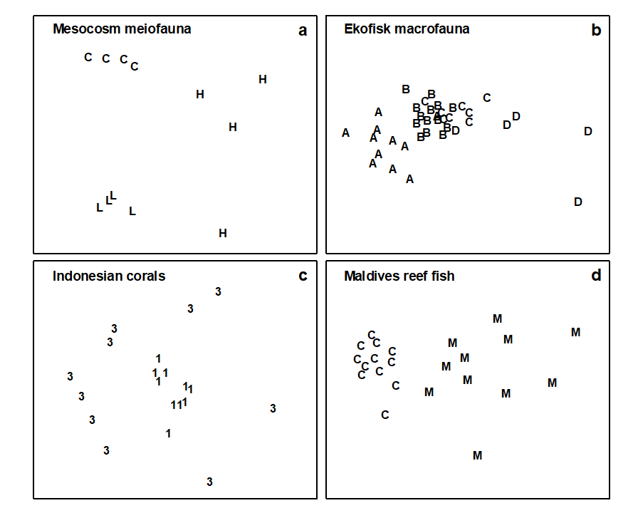
Fig. 15.4. Variability study {N, E, I, M}. Two-dimensional configurations for MDS ordinations of the four data sets. Treatment codes: a) H = High dose, L = Low dose, C = Controls; b) A–D are the station groupings by pollution load; c) 1 = 1981, 3 = 1983; d) M = Mined, C = Controls (stress: 0.08, 0.12, 0.11, 0.08).
It is possible to construct an index from the relative variability between impacted and control samples. One natural comparative measure of dispersion would be based on the difference in average distance among replicate samples for the two groups in the 2-d MDS configuration. However, this configuration is usually not an exact representation of the rank orders of similarities between samples in higher dimensional space. These rank orders are contained in the triangular similarity matrix which underlies any MDS. (The case for using this matrix rather than the distances is the same as that given for the ANOSIM statistic in Chapter 6.) A possible comparative Index of Multivariate Dispersion (IMD) would therefore contrast the average rank of the similarities among impacted samples ($\overline{r} _ t$) with the average rank among control samples ($\overline{r} _ c$) , having re-ranked the full triangular matrix ignoring all between-treatment similarities. Noting that high similarity corresponds to low rank similarity, a suitable statistic, appropriately standardised, is:
$$ IMD = 2 ( \overline{r} _ t - \overline{r} _ c ) / ( N _ t + N _ c) \tag{15.2} $$
where
$$ N _ c = n_ c (n _ c – 1)/2, \hspace{10mm} N _ t = n _ t (n _ t – 1)/2 \tag{15.3} $$
and $n _ c$, $n _ t$ are the number of samples in the control and treatment groups respectively. The chosen denominator ensures that IMD has maximum value of +1 when all similarities among impacted samples are lower than any similarities among control samples. The converse case gives a minimum for IMD of –1, and values near zero imply no difference between treatment groups.
In Table 15.2, IMD values are compared between each pair of treatments or conditions for the four examples. For the mesocosm meiobenthos, comparisons between the high dose and control treatments and the high dose and low dose treatments give the most extreme IMD value of +1, whereas there is little difference between the low dose and controls. For the Ekofisk macrofauna, strongly positive values are found in comparisons between the group D (most impacted) stations and the other three groups. It should be noted however that stations in groups C, B and A are increasingly more widely spaced geographically. Whilst groups B and C have similar variability, the degree of dispersion increases between the two outermost groups B and A, probably due to natural spatial variability. However, the most impacted stations in group D, which fall within a circle of 500 m diameter around the oil-field centre, still show a greater degree of dispersion than the stations in the outer group A which are situated outside a circle of 7 km diameter around the oil-field. Comparison of the impacted versus control conditions for both the Tikus Island corals and the Maldives reef-fish gives strongly positive IMD values. For the Maldives study, the mined sites were more closely spaced geographically than the control sites, so this is another example for which the increased dispersion resulting from the anthropogenic impact is ‘working against’ a potential increase in variability due to wider spacing of sites. Nonetheless, for both the Ekofisk and Maldives studies the increased dispersion associated with the impact more than cancels out that induced by the differing spatial scales.
Table 15.2. Variability study {N, E, I, M}. Index of Multivariate Dispersion (IMD) between all pairs of conditions.
 Study Study |
Conditions compared | IMD |
|---|---|---|
| Meiobenthos | High dose / Control | +1 |
| High dose / Low dose | +1 | |
| Low dose / Control | -0.33 | |
| Macrobenthos | Group D / Group C | +0.77 |
| Group D / Group B | +0.80 | |
| Group D / Group A | +0.60 | |
| Group C / Group B | -0.02 | |
| Group C / Group A | -0.50 | |
| Group B / Group A | -0.59 | |
| Corals | 1983 / 1981 | +0.84 |
| Reef-fish | Mined / Control reefs | +0.81 |
Application of the comparative index of multivariate dispersion (the MVDISP routine in PRIMER) suffers from the lack of any statistical framework for testing hypotheses of comparable variability among groups§. As given above, it is also restricted to the comparison of only two groups, though it can be extended to several groups in straightforward fashion. Let $\overline{r} _ i $ denote the mean of the $N _ i = n _ i ( n _ i – 1)/2$ rank similarities among the $n _ i$ samples within the ith group (i = 1, …, g), having (as before) re-ranked the triangular matrix ignoring all between-group similarities, and let N be the number of similarities involved in this ranking ($N = \sum _ i N _ i$). Then the dispersion sequence
$$ \overline{r} _ 1 /k, \hspace{3mm} \overline{r} _ 2 /k, \ldots \overline{r} _ g /k \tag{15.4} $$
defines the relative variability within each of the g groups, the larger values corresponding to greater within-group dispersion. The denominator scaling factor k is (N + 1)/2, i.e. simply the mean of all N ranks involved, so that a relative dispersion of unity corresponds to ‘average dispersion’. (If the number of samples is the same in all groups then the values in equation (15.4) will average 1, though this will not quite be the case if the {$n _ i$} are unbalanced.)
Table 15.3. Variability study {N, E, I, M}. Relative dispersion of the groups (equation 15.4) in each of the four studies.
| Meiobenthos | Control | 0.58 |
| Low dose | 0.79 | |
| High dose | 1.63 | |
| Macrobenthos | Group A | 1.34 |
| Group B | 0.79 | |
| Group C | 0.81 | |
| Group D | 1.69 | |
| Corals | 1981 | 0.58 |
| 1983 | 1.42 | |
| Reef-fish | Control reefs | 0.64 |
| Mined reefs | 1.44 |
As an example, the relative dispersion values given by (15.4) have been computed for the four studies (Table 15.3). This is complementary information to the IMD values; Table 15.2 provides the pairwise comparisons which follow the global picture in Table 15.3. The conclusions from the latter are, of course, consistent with the earlier discussion, e.g. the increase in variability at the outermost sites in the Ekofisk study, because of their greater geographical spread, being nonetheless smaller than the increased dispersion at the central, impacted stations.
These four examples all involve either experimental or spatial replication but a similar phenomenon can also be seen with temporal replication. Warwick, Ashman, Brown et al. (2002) report a study of macrobenthos in Tees Bay, UK, for annual samples (taken at the same two times each year) over the period 1973–96 {t}. This straddled a significant, and widely reported, phase shift in planktonic communities in the N Sea, in about 1987. The multivariate dispersion index (IMD), contrasting pre-1987 with post-1987, showed a consistent negative value (increase in inter-annual dispersion in later years) for each of six locations in Tees Bay, at each of the two sampling times (Table 15.4).
Table 15.4. Tees Bay macrobenthos {t}. Index of Multivariate Dispersion (IMD) between pre- and post-1987 years, before/after a reported change in N Sea pelagic assemblages.
| March | September | |
|---|---|---|
| Area 0 | –0.15 | –0.15 |
| Area 1 | –0.09 | –0.60 |
| Area 2 | –0.33 | –0.33 |
| Area 3 | –0.35 | –0.36 |
| Area 4 | –0.28 | –0.67 |
| Area 6 | –0.46 | –0.15 |
¶ We shall explore this data set in more detail in Chapter 16, in connection with the effect that choice of different resemblance measures has on the ensuing multivariate analyses. It is crucial to realise that this multivariate dispersion (seen in the MDS plot) represents variability in similarities among different replicate pairs and is not much influenced by, e.g., absolute variation in total cover. Euclidean distance, which is strongly influenced by the latter, shows the opposite pattern, with the replicates widely varying for 1981 and much tighter for 1983. Here, Bray-Curtis is driven by the turnover in species present (a concept ignored by Euclidean distance) in what is a sparse assemblage by 1983.
§ This is because there is no exact permutation process possible under a null hypothesis which says that dispersion is the same but location of the groups may differ. The only viable route to a test is firstly to estimate the locations of each group in some high-d ‘resemblance space’, and move those group centroids on top of each other. Having removed location differences, permuting the group labels becomes permissible under the null hypothesis. This is the procedure carried out by the PERMDISP routine in PERMANOVA+, Anderson (2006) . Like most tests in this add-on software it is therefore an approximate rather than exact permutation test (because of the estimation step) and is semi-parametric not non-parametric (based on similarities themselves not their ranks).
15.4 Breakdown of seriation
Clear-cut zonation patterns in the form of a serial change in community structure with increasing water depth are a striking feature of intertidal and shallow-water benthic communities on both hard and soft substrata. The causes of these zonation patterns are varied, and may differ according to circumstances, but include environmental gradients such as light or wave energy, competition and predation. None of these mechanisms, however, will necessarily give rise to discontinuous bands of different assemblages of species, which is implied by the term zonation, and the more general term seriation is perhaps more appropriate for this pattern of community change, zonation (with discontinuities) being a special case.
Many of the factors which determine the pattern of seriation are likely to be modified by disturbances of various kinds. For example, dredging may affect the turbidity and sedimentation regimes and major engineering works may alter the wave climate. Elimination of a particular predator may affect patterns which are due to differential mortality of species caused by that predator. Increased disturbance may also result in the relaxation of interspecific competition, which may in turn result in a breakdown of the pattern of seriation induced by this mechanism. Where a clear sequence of community change along transects is evident in the undisturbed situation, the degree of breakdown of this sequencing could provide an index of subsequent disturbance. Clarke, Warwick & Brown (1993) have described a simple non-parametric index of multivariate seriation, and applied it to a study of dredging impact on intertidal coral reefs at Ko Phuket, Thailand {K}.
In 1986, a deep-water port was constructed on the SE coast of Ko Phuket, involving a 10-month dredging operation. Three transects were established across nearby coral reefs (Fig. 15.5), transect A being closest to the port and subject to the greatest sedimentation, partly through escape of fine clay particles through the southern containing wall. Transect C was some 800 m away, situated on the edge of a channel where tidal currents carry sediment plumes away from the reef, and transect B was expected to receive an intermediate degree of sedimentation. Data from surveys of these three transects, perpendicular to the shore, are presented here for 1983, 86, 87 and 88 (see Chapter 16 for later years). Line-samples of 10m were placed parallel to the shore at 10m intervals along the main transect from the inner reef flat to the outer reef edge, 12 lines along each of transects A and C and 17 along transect B. The same transects were relocated each year and living coral cover of each species recorded.

Fig. 15.5. Ko Phuket corals {K}. Map of study site showing locations of transects, A, B and C.
The basic data were root-transformed and Bray-Curtis similarities calculated between every pair of samples within each year/transect combination (C was not surveyed in 1986); the resulting triangular similarity matrices were then input to non-metric MDS (Fig. 15.6). By joining the points in an MDS, in the order of the samples along the inshore-to-offshore transect, one can visualise the degree of seriation, that is, the extent to which the community changes in a smooth and regular fashion, departing ever further from the community at the start of the transect. A measure of linearity of the resulting sequence could be constructed directly from the location of the points in the MDS. However, this could be misleading when the stress is not zero, so that the pattern of relationships between the samples cannot be perfectly represented in 2 dimensions; this will often be the case, as with some of the component plots in Fig. 15.6¶. Again, a better approach is to work with the fundamental similarity matrix that underlies the MDS plots, of whatever dimension.
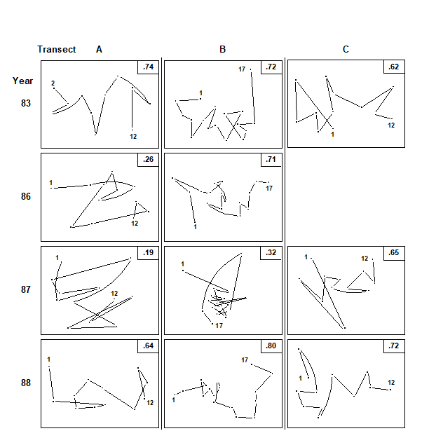
Fig. 15.6. Ko Phuket corals {K}. MDS ordination of the changing coral communities (species cover data) along three transects (A to C) at four times (1983 to 1988). The lines indicate the degree of seriation by linking successive points along a transect, from onshore (1) to offshore samples (12 or 17); $\rho$ values (seriation statistic, IMS) are at top right. Sample 1 from transect A in 1983 is omitted (see text) and no samples were taken for transect C in 1986 (reading across rows, stress = 0.10, 0.11, 0.09; 0.10, 0.11; 0.08, 0.14, 0.11; 0.07, 0.09, 0.10).
The index of multivariate seriation (IMS) proposed is therefore defined as a Spearman correlation coefficient ($\rho _ s$, e.g. Kendall (1970) , see also equation 6.3) computed between the corresponding elements of two triangular matrices of rank ‘dissimilarities’. The first is that of Bray-Curtis coefficients calculated for all pairs from the n coral community samples (n = 12 or 17 in this case). The second is formed from the inter-point distances of n points laid out, equally-spaced, along a line. If the community changes exactly match this linear sequence (for example, sample 1 is close in species composition to sample 2, samples 1 and 3 are less similar; 1 and 4 less similar still, up to 1 and 12 having the greatest dissimilarity) then the IMS has a value $\rho = 1$. If, on the other hand, there is no discernible biotic pattern along the transect, or if the relationship between the community structure and distance offshore is very non-monotonic – with the composition being similar at opposite ends of the transect but very different in the middle – then $\rho$ will be close to zero. These near-zero values can be negative as well as positive but no particular significance attaches to this.
A statistical significance test would clearly be useful, to answer the question: what value of $\rho$ is sufficiently different from zero to reject the null hypothesis of a complete absence of seriation? Such an (exact) test can be derived by permutation in this case. If the null hypothesis is true then the labelling of samples along the transect (1, 2, …, n) is entirely arbitrary, and the spread of $\rho$ values which are consistent with the null hypothesis can be determined by recomputing its value for permutations of the sample labels in one of the two similarity matrices (holding the other fixed). For T randomly selected permutations of the sample labels, if only t of the T simulated $\rho$ values are greater than or equal to the observed $\rho$, the null hypothesis can be rejected at a significance level of 100(t+1)/(T+1)%.†
In 1983, before the dredging operations, MDS configurations (Fig.15.6) indicate that the points along each transect conform rather closely to a linear sequence, and there are no obvious discontinuities in the sequence of community change (i.e. no discrete clusters separated by large gaps); the community change follows a quite gradual pattern. The values of $\rho$ are consequently high (Table 15.5), ranging from 0.62 (transect C) to 0.72 (transect B).
Table 15.5. Ko Phuket corals {K}. Index of Multivariate Seriation ($\rho$) along the three transects, for the four sampling occasions. Figures in parentheses are the % significance levels in a permutation test for absence of seriation (T = 999 simulations).
| Year | Transect A | Transect B | Transect C |
|---|---|---|---|
| 1983 | 0.65 (0.1%) | 0.72 (0.1%) | 0.62 (0.1%) |
| 1986 | 0.26 (3.8%) | 0.71 (0.1%) | – |
| 1987 | 0.19 (6.4%) | 0.32 (0.2%) | 0.65 (0.1%) |
| 1988 | 0.64 (0.1%) | 0.80 (0.1%) | 0.72 (0.1%) |
The correlation with a linear sequence is highly significant in all three cases. Note that in the 1983 MDS for transect A, the furthest inshore sample has been omitted; it had very little coral cover and was an outlier on the plot, resulting in an unhelpfully condensed display of the remaining points. The MDS has therefore been run with this point removed§. There is no similar technical need, however, to remove this sample from the $\rho$ calculation; this was not done in Table 15.5 though doing so would increase the $\rho$ value from 0.65 to 0.74 (as indicated in Fig. 15.6).
On transect A, subjected to the highest sedimentation, visual inspection of the MDS gives a clear impression of the breakdown of the linear sequence for the next two sampling occasions. The IMS is dramatically reduced to 0.26 in 1986, when the dredging operations commenced, although the correlation with a linear sequence is still just significant (p=3.8%). By 1987, $\rho$ on this transect is further reduced to 0.19 and the correlation with a linear sequence is no longer significant. On transect B, further away from the dredging activity, the loss of seriation is not evident until 1987, when the sequencing of points on the MDS configureation breaks down and the IMS is reduced to 0.32, although the latter is still significant (p=0.2%). Note that the MDS plots of Fig. 15.6 may not tell the whole story; the stress values lie between 0.07 and 0.14, indicating that the 2-dimensional pictures are not perfect representations. The largest stress is, in fact, that for transect B in 1987, so that the seriation that is still detectable by the test is only imperfectly seen in the 2-dimensional plot. It is also true that the increased number of points (17) on transect B, in comparison with A and C (12), will lead to a more powerful test. Essentially though what the test is picking up is a tendency for nearby samples on the transect to have more similar assemblages and one should bear in mind in interpreting such analyses that (as with the earlier ANOSIM test) it is the value of the statistic itself which gives the key information here: values around 0.6 or more will only be obtained if there is a clear serial trend in the samples. Smaller, but still significant values could result from serial autocorrelation, which the test will have some limited power to detectȹ.
On transect C there is no evidence of the breakdown of seriation at all, either from the $\rho$ values or from inspection of the MDS plot. By 1988 transects A and B had completely recovered their seriation pattern, with $\rho$ values highly significant (p<0.1%) and of similar size to those in 1983, and clear sequencing evident on the MDS plots. There was clearly a graded response, with a greater breakdown of seriation occurring earlier on the most impacted transect, some breakdown on the middle transect but no breakdown at all on the transect least subject to sedimentation.
Overall, the breakdown in the pattern of seriation was due to the increase in distributional range of species which were previously confined to distinct sections of the shore. This is commensurate with the disruption of almost all the types of mechanism which have been invoked to explain patterns of seriation, and gives us no clue as to which of these is the likely cause.
¶ Even where the stress is low, the well-known arch effect, Seber (1984) , mitigates against a genuinely linear sequence appearing in a 2-d ordination as a straight line; see the footnote on page 11.3. Or to put it a simpler way, given the whole of 2-d space in which to place points which are essentially in sequence (i.e. the distance between points 1 and 2 is less than that between 1 and 3 which is less than between 1 and 4 etc), it is clear that points can ‘snake around’ (without coiling!) in that 2-d space in a large number of possible ways, few of which will end up looking like a straight line. Transect B in Years 83, 86 and 88 are a good case in point: none will be well fitted by a straight line regression on the MDS plot but they clearly have a very strong serial trend.
† The calculations for the tests were carried out using the PRIMER RELATE routine, which is examined in more detail, and in more general form below, when this particular example is concluded. It has been referred to previously in Chapters 6 & 11 ($\rho$ statistic).
§ The problem is discussed on page 5.8 and the solution presented there, mixing a small amount of mMDS stress to the nMDS stress would have been an alternative, effective way of dealing with this.
ȹ The distinction between trend and serial autocorrelation in univariate statistics can be somewhat arbitrary. One can often model a time series just as convincingly by (say) a cubic polynomial response with a simple independent error term as by a simple linear fit with an autocorrelated error structure: which we choose is sometimes a matter of convention. Here, where the non-parametric framework steers clear of any parametric modelling, the test needs to be realistic in ambition: it can demonstrate an effect, and the size of that effect ($\rho$) and the accompanying MDS plot guides interpretation: large values imply a strong serial trend.
15.5 Model matrices & ‘RELATE’ tests
The form of the seriation statistic is simply a matrix correlation coefficient (e.g. equation 11.3) between the unravelled entries of the similarity matrix of the biotic samples and a model distance matrix defined, in this case from equi-spaced points on a line:

Correlation coefficients available with the PRIMER RELATE routine are three non-parametric options: Spearman, equation (11.3); Kendall’s $\tau$ ( Kendall (1970) ); weighted Spearman (11.4); and one measure which uses the similarities themselves rather than their ranks: the standard product-moment or Pearson correlation, (2.3). The latter is the form of matrix correlation first defined by Mantel (1967) , in an epidemiological context. The Spearman coefficient $\rho$ is a natural choice for our rank-based philosophy and has an interesting affinity with the ordered ANOSIM statistic, $R ^ O$, discussed on page 6.10, which builds the same model matrix of serial trend (with or without replication, see later). This can, of course, be seriation in time rather than space, so this form of RELATE test provides a useful means of testing and quantifying the extent of a time trend – perhaps an inter-annual drift away of an assemblage from its initial state, through gradual processes such as climate change.
15.6 Examples
Example: Tees Bay macrofauna
Fig. 15.7 shows the nMDS plot for the inter-annual macrofauna samples (282 species) collected every September from 1973 to 1976 in four areas of Tees Bay ({t}, see Fig. 6.17 for map, and individual MDS plots for each area). The current plot uses averages of the 4th-root transformed counts over the four areas (and the two sites within each area), and Bray-Curtis similarities, to obtain an overall picture of the time trend in the benthos. Relating the Bray-Curtis matrix to a triangular matrix of a seriation model, as shown schematically above, the (matrix) Spearman rank correlation ($\rho$) takes a high value of 0.68. Though the stress in the MDS is not negligibly low, the strong time trend seen in this statistic is very evident in the plot. Notice again that is it not at all necessary for the plot to take the form of a straight line to obtain a high $\rho$ value: the statistic is much more general than this and the approximations inherent in any low-d ordination are avoided by direct correlation of the observed and modelled resemblance matrices. High $\rho$ values are triggered by any continuing movement of the community away from its initial state.
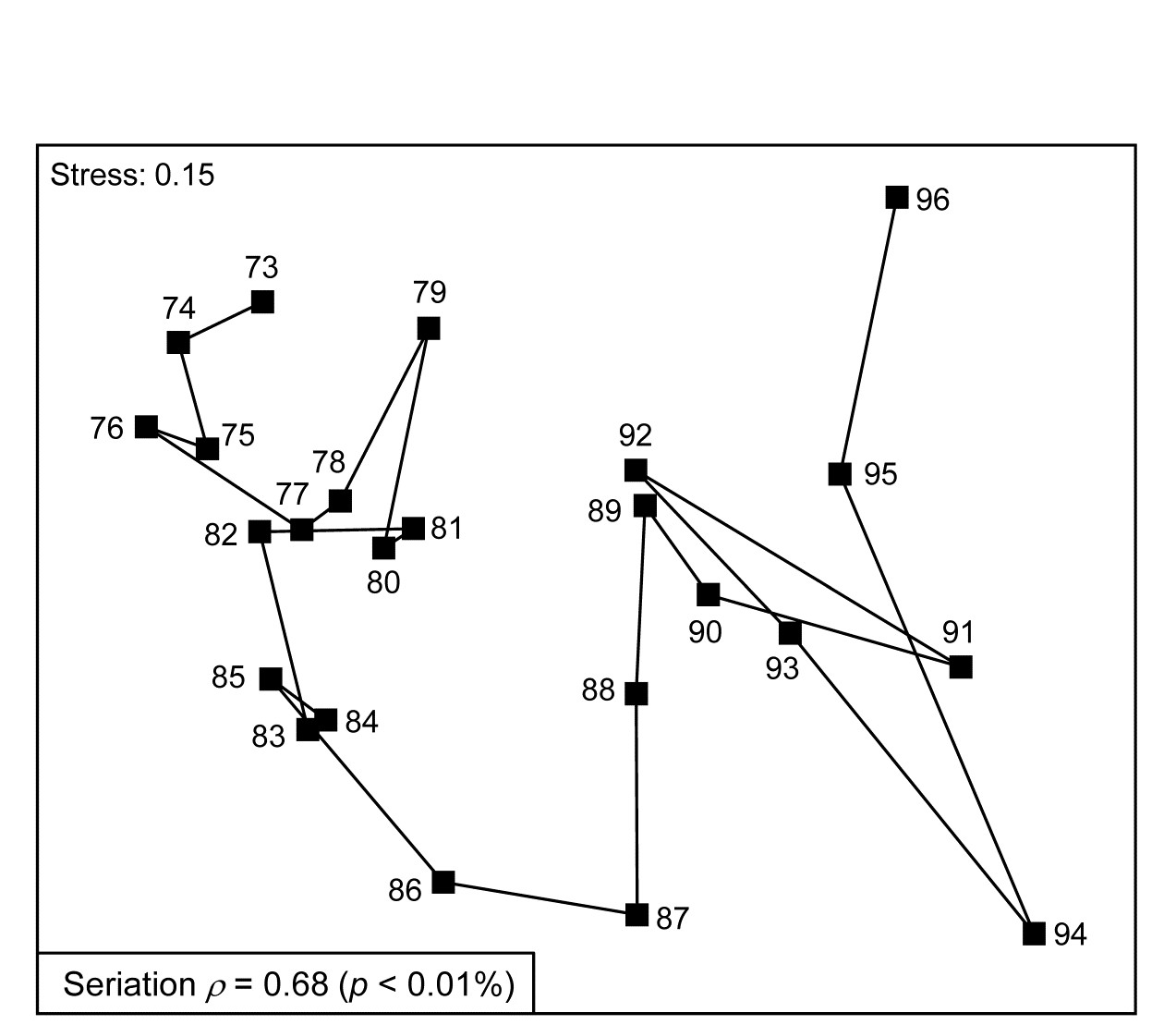
Fig. 15.7. Tees Bay macrofauna {t}. MDS plot of inter-annual time trend in averaged data over 4 areas (and 2 sites per area), for September samples, based on 4th-root transformed counts of 282 species and Bray-Curtis similarities among averaged samples.
As explained above, the hypothesis test available is only of the null hypothesis H$_ 0$: $\rho = 0$, that there is no link of the assemblage to such a serial time sequence, and the null distribution is obtained by recalculating $\rho$ for a large number of random reassignments of the 24 year numbers to the 24 samples. (Note that this is not a test of the hypothesis $\rho = 1$, of a perfect time trend – that is a common misunderstanding!). Here, unsurprisingly, the observed sequence gives a higher $\rho$ than any of 9999 such permutations (p << 0.1%) and is never higher here than about $\rho$ = 0.3 by chance (the large number of years gives a ‘powerful’ test).
The matrix correlation idea can be much more general than seriation, as was seen in Chapter 11, where it was used in the BEST routine to link biotic dissimilarity to a distance calculated from environmental variables. Model matrices can therefore be viewed as just special cases of abiotic data which define an a priori structure, an (alternative) hypothesis which we erect as a plausible model for the biotic data. We wish then to do two things: to test the null hypothesis that there is no link of the data to the hypothesised model, and if rejected, to interpret the size of the correlation $\rho$ of the data to the model.
The model matrix for the Phuket coral data was based on simple physical distance between the 10m-spaced transect positions down the shore. This generalises in an obvious way to the physical distance between all pairs of sampling locations in a geographical layout (indeed this was the distance matrix used by Mantel for his work on clustering of cancer incidences). The test and $\rho$ statistic then quantify how strongly related observed assemblages are to mutual proximity of the samples, and the model matrix can be created by inputting simple x, y co-ordinates (e.g. the decimalised latitude-longitude) to a resemblance calculation of non-normalised Euclidean distance.
Example: Loch Creran/Etive macrofauna
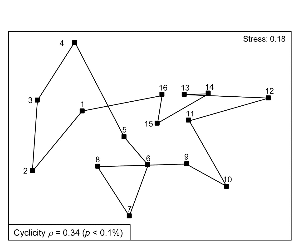
Fig. 15.8. Creran & Etive sea-loch macrofauna {c}. MDS of species abundance data from sub-tidal samples taken at 16 equally-spaced locations on the circumference of a circle (in an unperturbed environment). Significant (albeit weak) match to a cyclic model matrix.
Somerfield & Gage (2000) describe grab sampling of subtidal soft sediments in Scottish sea-lochs, by a vessel positioning at points equidistant (~50m) from a moored buoy, giving 16 equal-spaced samples around a 100m diameter circle (samples numbered 1-16). An MDS ordination from this data set is seen in Fig. 15.8 and while again the stress is high, so the 2-d MDS is not very reliable, there is certainly a suggestion that the samples, joined in their order of sampling, around the circle, match this spatial layout. A model matrix from a serial trend is no longer appropriate of course; instead it will be of the following general form (but illustrated only for 6 points around a circle)¶.
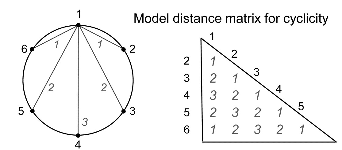
For equal-spaced points round a circle, the inter-point distances shown are not physically accurate – they are chords of a circle, and if that is of radius 1, the actual distances would be 1, 1.73 ($= \sqrt{3}$) and 2, rather than 1, 2 and 3 – but the model matrix is shown with distances 1, 2 and 3 because a Spearman correlation is only a function of the rank orders of the distances.
The matching coefficient of the assemblage (dis)similarities to this distance coefficient is $\rho = 0.34$, and this was larger than produced by any of 999 random permutations of the labels, hence the null hypothesis of no match can be rejected (at p < 0.1%), on a test designed for an alternative hypothesis of cyclicity.
However, rather than a spatial context, a cyclic model matrix is much more likely to be useful in a temporal study, e.g. where seasonality (or perhaps diurnal data) is involved. A data set with monthly levels 1-12, for January to December, would fit poorly to a seriation since the latter would dictate that December was the most dissimilar month to January. An example of bi-monthly sampling, where a test for a hypothesis of no seasonality is not a foregone conclusion, is provided by the Exe estuary nematode data met extensively in Chapters 5 and 11, and also in Chapter 7.
Example: Exe estuary nematodes
Fourth-root transformed nematode counts from 174 species are averaged over the 19 sampling sites of the Exe estuary study {X}, separately for each of the 6 bi-monthly sampling times through a single year. (Note that most previous analyses in this manual have used the data averaged over the months, separately for the sites, though an exception is Fig. 6.12). The question is simply whether there is any overall demonstration of seasonal pattern in these 6 meiofaunal community samples? The model matrix is now exactly that shown immediately to the left and the Spearman correlation of Bray-Curtis dissimilarities with this matrix is 0.21. The evidence in Fig. 15.9 for any such cyclic pattern is unconvincing, either in the MDS or in the formal RELATE test (p = 20%, see inset, where the jagged null distribution is a result of the small number of distinct permutations of the 6 numbers, i.e. 5! = 120).

Fig. 15.9. Exe estuary nematodes {X}. nMDS on Bray-Curtis similarities from counts of 174 species, 4th-root transformed then averaged over the 19 locations, for each of 6 bi-monthly sampling times over one year (1-6). Inset: null distribution for test of cyclicity (r=0.21).
Seriation with replication
Quite commonly, there will be interest in testing for a serial trend in the presence of replicate observations at each of the points in time or space (or at ordered treatment levels etc). This is precisely the problem that was posed towards the end of Chapter 6 (page 6.10 onwards) in setting up the ordered ANOSIM tests. There are now ordered groups of samples (A, B, C, …), and the null hypothesis ‘H$_ 0$: A=B=C=…’ that the groups are indistinguishable is not tested against a non-specific alternative ‘H$_ 1$: A, B, C, … differ’ but against the ordered seriation model ‘H$_ 1$: A<B< C …’. More detail is given on page 6.10 to page 6.12 , but the only difference here is that instead of using the generalised ANOSIM statistic $R ^ 0$, the slope of the regression line of the ranks {$r _ i$} in the (biotic) dissimilarity matrix against the ranks {$s _ i$} in the model matrix, we use here their correlation $\rho$ (this is Pearson correlation on the ranks, i.e. Spearman on the matrices).

The simple form of seriation with replication (the model matrix for which is seen above, illustratively, for 3 groups A, B, C, with 2 replicates in groups A and C, and 3 replicates in B), was extensively studied by
Somerfield, Clarke & Olsgard (2002)
and illustrated by further Norwegian oilfield benthic data from the N Sea, {g}.
Example: Gullfaks oilfield macrofauna
Routine monitoring of soft-sediment macrobenthos around all the Norwegian oilfields typically involves sites radiating in several directions (usually 4) from the centre of each field (as in the Ekofisk study, see Fig. 10.6), but for analysis purposes broadly grouped into distance classes. For the two oilfields: GullfaksA (16 sites, 1989 data) and GullfaksB (12 sites, 1993), 3 groups were defined as C: <1km, B: ~1km, A: > 1km from the centre of drilling activity, each consisting of between 4 and 6 replicate sites. These are shown as differing symbols and shading on their faunal MDS plots in Fig. 15.10. Unlike the Ekofisk data, where the oilfield had been operating for longer, the group differences are less clear-cut, and differences are not significantly established in unordered ANOSIM tests.
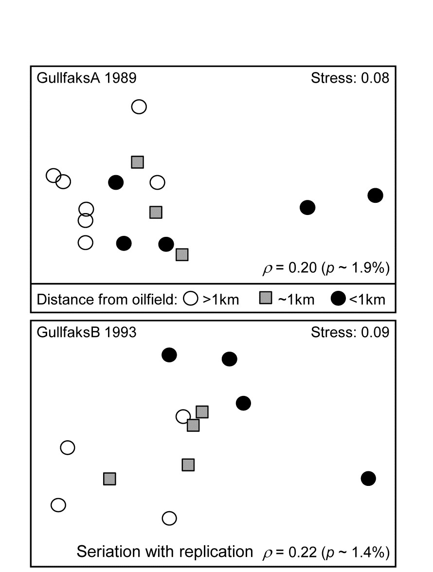
Fig. 15.10. Gullfaks oilfields, macrofauna {g}. nMDS on Bray-Curtis similarities from transformed species counts for sites in 3 distance groups A: >1km, B: ~1km, C: <1km from the oilfield centres. Both show a significant left to right progression, with seriation statistics $\rho$ =0.20 and $\rho$ =0.22 for GullfaksA and GullfaksB fields respectively.
However, when tested against the ordered alternative, using the seriation with replication schematic (above) the $\rho$ values of 0.20 and 0.22 are both significant at about the p < 2% level. The issue here is one of power of the test. As Somerfield, Clarke & Olsgard (2002) show, where a test against an ordered alternative is relevant, it will have more power to reject the null hypothesis (‘no group differences’) in favour of that alternative†. The improved power always comes at a price though, namely the likely inability to detect an alternative which is not the postulated model matrix. Thus, in Fig. 15.10, B is generally intermediate between A and C, and this is as postulated. If the benthic community is distinct at differing distances from the oilfield as a result of dilution of contaminants coming from the centre§, then a situation in which groups A and C have indistinguishable benthic assemblages but B has a different one would not be interpretable, and would be discounted as a ‘fluke’. If we are happy to forgo the prospect of ever detecting such a case then it makes sense to focus the statistic on alternatives that are of interest, and thereby gain power.
Constrained (‘2-way’) RELATE tests
Just as was seen with the BEST procedure in Chapter 11 (page 11.5), it is straightforward to remove the effect of a further (crossed) factor when testing similarities against a model matrix (or any secondary matrix). The $\rho$ statistic is calculated separately within each level of the ‘nuisance’ factor, so that any effect of the latter is removed, and the resulting $\rho$ statistics then averaged. The same procedure is carried out for the permutations under the null hypothesis, i.e. it is a constrained permutation in which labels are only permuted within the levels of the second (nuisance) factor, just as in 2-way ANOSIM or its ordered form (page 6.5 and page 6.12). However, the ordered ANOSIM tests in PRIMER v7 only implement the seriation model (with or without replication), so the following RELATE example illustrates a 2-factor case where a cyclic test is needed on (replicated) seasons, having removed regional differences in the assemblages, {l}.
Example: Leschenault estuarine fish
Veale, Tweedley, Clarke et al. (2014) describe nearshore trawls for fish abundance (43 species) in a microtidal W Australian estuary, with freshwater inflow only near the estuary mouth (Basal region, B) and thus a reverse salinity gradient increasing through its Lower (L), Upper (U) and Apex (A) regions. That region has a strong effect on fish communities is evident from the MDS of Fig. 15.11b, for 6-8 replicate samples (both spatially, in regions, and temporally, across years) from each of 16 combinations of 4 seasons and 4 regions. There is some suggestion from Fig. 15.11a (the same MDS but showing seasons) of a seasonal effect, but this is hard to discern, given also the strong regional effect.
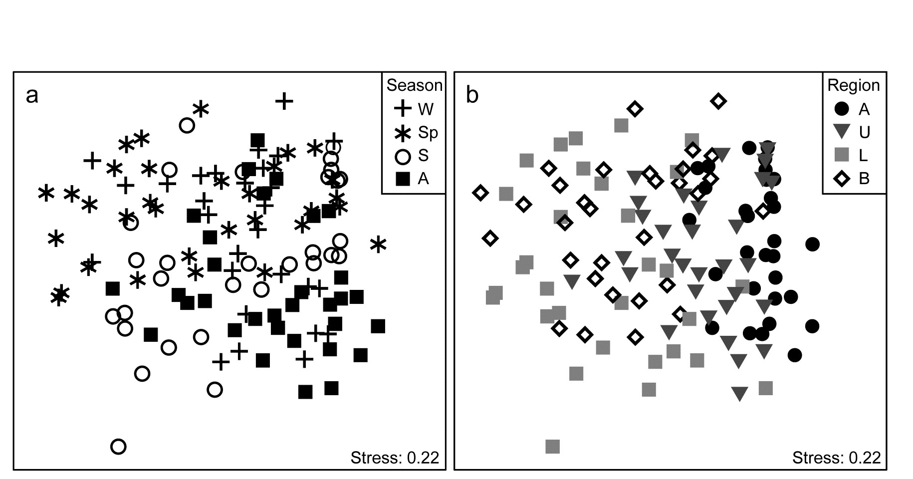
Fig. 15.11. Leschenault estuary fish {l}. nMDS from Bray-Curtis on dispersion weighted then $\sqrt{}$-transformed samples of counts from 43 species, of sites within the four regions (Apex, Upper, Lower, Basal) over two years and in all seasons of each year (Winter, Spring, Summer and Autumn). a) and b) are the same MDS but indicate samples from seasons & regions respectively.
The conditional test for seasonality fits the model matrix on page 15.6, but for only 4 not 6 times (Autumn, Winter, Spring, Summer) and with replication. (A test without replication is possible but this really needs to be for monthly or bimonthly data rather than just four seasons, since there are only 3! = 6 distinct permutations from a single set of 4 times). The $\overline{\rho}$ statistic, averaging the cyclicity (seasonality) $\rho$ values, given by each region separately, is only 0.27, indicating the high replicate variability (seen in Fig. 15.11a and b), but this is strongly significantly different from zero (p<<0.01%) since the permutations never came close to producing an average $\rho$ larger than 0.1. That there is a clear seasonal effect, consistently across regions, can be seen (as must always be done, and rarely is!) by averaging over the temporal and spatial replicates to obtain the 16-sample nMDS of Fig. 15.12.
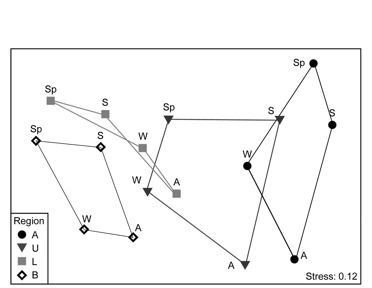
Fig. 15.12. Leschenault estuary fish {l}. nMDS from Bray-Curtis for averages over all samples (previously dispersion weighted then transformed, page 9.6) from 4 regions over 4 seasons. Regions align left to right in increasing salinity up the estuary, clearly with parallel seasonal cycles.
¶ The PRIMER RELATE routine gives three options: match to a simple seriation (distance matrix of the type on page 15.5), simple cyclicity (distance matrix as seen here) or to any other supplied triangular matrix (a further model matrix, or possibly a second biotic resemblance matrix, e.g. testing and quantifying the match of reef fish community structure to the coral reef assemblages on which they are found). A separate routine on the Tools menu, Model Matrix, allows the user to create more complex models, for seriation or cyclicity where spacing is unequal or where there are replicates at each point. These are specified by numeric levels of a factor. E.g. though this simple 6-point circular model is automatically catered for by RELATE, recreating it using the Model Matrix routine needs a factor with levels in (0,1), taken to be the same point at the start and end of the circle, i.e. use levels 0, 0.167, 0.333, 0.5, 0.667, 0.833 for the samples 1, 2, 3, 4, 5, 6.
† This is certainly true of the analogue in univariate statistics (see Somerfield, Clarke & Olsgard (2002) ), e.g. the choice between ANOVA and linear regression when treatment levels (with replication) are numeric. Regression is always the more powerful, though it would completely miss, for example, a hormesis response that ANOVA would detect. Power is a much more difficult concept in multivariate space but Somerfield, Clarke & Olsgard (2002) demonstrate a similar result for unordered ANOSIM vs RELATE (i.e. ordered ANOSIM) in some special cases, by simulation from observed alternatives to the null of ‘no change’.
§ Or a number of other causal mechanisms to do with existence of the oilfield that might be tricky to distinguish by biotic observational data alone, e.g. a change in the sediment structure resulting from deposition of finer grained drilling muds, maybe disruption of current flows, even reduced commercial fishing pressure etc.