Chapter 17: Biodiversity and dissimilarity measures based on relatedness of species

17.1 Species richness disadvantages
17.2 Average taxonomic diversity and distinctness
17.3 Examples: Ekofisk oil-field and Tees Bay soft-sediment macrobenthos
17.4 Other relatedness measures
17.5 ‘Expected distinctness’ tests
17.6 Example: UK free-living nematodes
17.7 Example: N Europe groundfish surveys
17.8 Variation in taxonomic distinctness, $\Lambda ^ +$
17.9 Joint (AvTD, VarTD) analyses
17.10 Concluding remarks on taxonomic distinctness
17.11 Taxonomic dissimilarity
17.12 Examples

17.1 Species richness disadvantages

Chapter 8 discussed a range of diversity indices based on species richness and the species abundance distribution. Richness (S) is widely used as the preferred measure of biological diversity (biodiversity) but it has some major drawbacks, many of which apply equally to other diversity indices such as H$^\prime$, H, J$^\prime$, etc.

Observed richness is heavily dependent on sample size/effort. In nearly all marine contexts, it is not possible to collect exhaustive census data. The assemblages are sampled using sediment cores, trawls etc, and the ‘true’ species richness of a station is rarely fully represented in such samples. For example, Gage & Coghill (1977) describe a set of contiguous core samples taken for macrobenthic species in a Scottish sea-loch. A species-area plot (or accumulation curve) which illustrates how the number of different species detected increases as the samples are accumulated^¶, shows that, even after 64 replicate samples are taken at this single locality, the observed number of species is still rising.

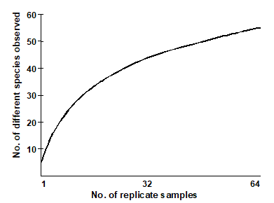
“The harder you look, the more species you find” is fundamental to much biological sampling and the asymptote of accumulation curves is rarely reached. Observed species richness S is therefore highly sensitive to sample size and totally non-comparable across studies involving unknown, uncontrolled or simply differing degrees of sampling effort. The same is true, to a lesser extent, of many other standard diversity indices. Fig. 17.1 shows the effect of increasing numbers of individuals on the values of some of the diversity indices defined in Chapter 8. This is a sub-sampling study, selecting different numbers of individuals at random from a single, large community sample. The only index to demonstrate a lack of bias in mean value is Simpson diversity, given here in the form $1 - \lambda ^ \prime$, see equation (8.4). Comparison of richness, Shannon, evenness, Brillouin etc values for differing sample sizes is clearly problematic.

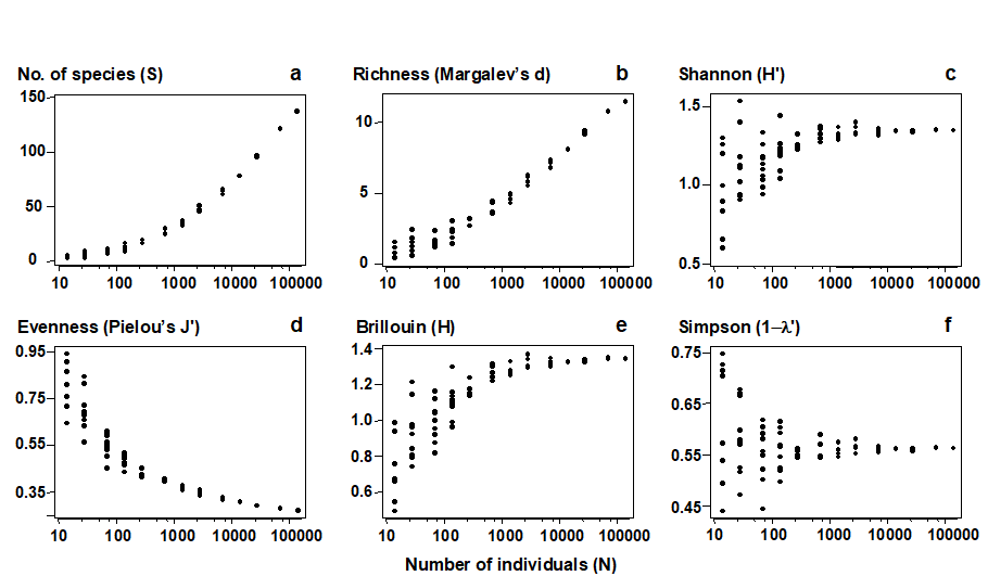
Fig. 17.1. Amoco-Cadiz oil spill {A}, pooled pre-impact data. Values of 6 standard diversity indices (y-axis, see Chapter 8 for definitions), for simulated samples of increasing numbers of individuals (x-axis, log scaled), drawn randomly without replacement from the full set of 140,344 macrobenthic organisms.

Species richness does not directly reflect phylogenetic diversity. “A measure of biodiversity of a site ought ideally to say something about how different the inhabitants are from each other” ( Harper & Hawksworth (1994) ). It is clear that a sample consisting of 10 species from the same genus should be seen as much less biodiverse than another sample of 10 species, all of which are from different families: genetic, phylogenetic or, at least, taxonomic relatedness of the individuals in a sample is the key concept which is developed in this chapter, into practical indices which genuinely reflect biodiversity and are robust to sampling effort variations.
No statistical framework exists for departure of S from ‘expectation’. Whilst observed species richness measures can be compared across sites (or times) which are subject to strictly controlled and equivalent sampling designs, there is no sense in which the values of S can be compared with some absolute standard, i.e. we cannot generally answer the question “what do we expect the richness to be at this site?”, in the absence of anthropogenic impact, say.
The response of S to environmental degradation is not monotonic. Chapter 8 discusses the well-established paradigm (see Wilkinson (1999) and references therein) that, under moderate levels of disturbance, species richness may actually increase, before decreasing again at higher impact levels. It would be preferable to work with a biological index whose relation to the degree of perturbation was purely monotonic (increasing or decreasing, but not both).
Richness can vary markedly with differing habitat type. Again, the ideal would be a measure which is less sensitive to differences in natural environmental variables but is responsive to anthropogenic disturbance.

^¶ This uses the Species-Accumulation Plot routine in PRIMER, with the option of plotting the curve in the presented sample order or (as here) randomising that order a large number of times. In the latter case, the resulting curves are averaged to obtain a smooth relationship of average number of species for each number of replicates. The routine also computes several standard extrapolation models which attempt to predict the asymptotic number of species that would be found for an infinity of samples from the same (closed) location. Included are Chao estimators, jacknife and bootstrap techniques, see Colwell & Coddington (1994) .

17.2 Average taxonomic diversity and distinctness

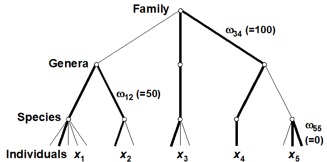
Two measures, which address some of the problems identified with species richness and the other diversity indices, are defined by Warwick & Clarke (1995b) . They are based not just on the species abundances (denoted by $x _ i$, the number of individuals of species i in the sample) but also the taxonomic distances ($\omega _ {ij}$), through the classification tree, between every pair of individuals (the first from species i and the second from species j). For a standard Linnean classification, these are discrete distances, the simple tree below illustrating path lengths of zero steps (individuals from the same species), one step (same genus but different species) and two steps (different genera)^¶. Clarke & Warwick (1999) advocate a simple linear scaling whereby the largest number of steps in the tree (two species at greatest taxonomic distance apart) is set to $\omega = 100$. Thus, for a sample consisting only of the 5 species shown, the path between individuals in species 3 and 4 is $\omega _ {34} = 100$, between species 1 and 2 is $\omega _ {12} = 50$, between two individuals of species 5 is $\omega _ {55} = 0$, etc.

Average taxonomic diversity of a sample is then defined ( Warwick & Clarke (1995b) ) as: $$ \Delta = \left[ \sum \sum _ {i < j} \omega _ {ij} x _ i x _ j \right] / \left[ N (N – 1)/2 \right] \tag{17.1} $$

where the double summation is over all pairs of species i and j (i,j = 1, 2, …, S; i<j), and $N = \sum _ i x _ i$, the total number of individuals in the sample. $\Delta$ has a simple interpretation: it is the average ‘taxonomic distance apart’ of every pair of individuals in the sample or, to put it another way, the expected path length between any two individuals chosen at random.

Note also that when the taxonomic tree collapses to a single-level hierarchy (all species in the same genus, say), $\Delta$ becomes

$$ \Delta ^ \circ = \left[ 2 \sum \sum _ {i < j} p _i p _ j \right] / ( 1 - N ^ {-1} ) = \left( 1 - \sum _ i p _ i ^ 2 \right) / ( 1 - N ^ {-1} ) \tag{17.2}$$ $ \hspace{117pt}$ where $p _ i = x _ i / N $

which is a form of Simpson diversity. The Simpson index is actually defined from the probability that any two individuals selected at random from a sample belong to the same species ( Simpson (1949) ). $\Delta$ is therefore seen to be a natural extension of Simpson, from the case where the path length between individuals is either 0 (same species) or 100 (different species) to a more refined scale of intervening relatedness values (0 = same species, 20 = different species in the same genera, 40 = different genera but same family, etc).^† It follows that $\Delta$ will often track Simpson diversity fairly closely. To remove the dominating effect of the species abundance distribution {$x _ i$}, leaving a measure which is more nearly a pure reflection of the taxonomic hierarchy, Warwick & Clarke (1995b) proposed dividing $\Delta$ by the Simpson index $\Delta ^ \circ$ to give average taxonomic distinctness $$ \Delta ^ \ast = \left[ \sum \sum _ {i < j} \omega _ {ij} x _ i x _ j \right] / \left[\sum \sum _ {i < j} x _ i x _ j \right] \tag{17.3} $$ Another way of thinking of this is as the expected taxonomic distance apart of any two individuals chosen at random from the sample, provided those two individuals are not from the same species.

A further form of the index, exploited greatly in what follows, takes the special case where quantitative data is not available and the sample consists simply of a species list (presence/absence data). Both $\Delta$ and $\Delta ^ \ast$ reduce to the same coefficient

$$ \Delta ^ + = \left[ \sum \sum _ {i < j} \omega _ {ij} \right] / \left[ S (S - 1) / 2 \right] \tag{17.4} $$

where S, as usual, is the observed number of species in the sample and the double summation ranges over all pairs i and j of these species (i<j). Put simply, the average taxonomic distinctness (AvTD) $\Delta ^ +$ of a species list is the average taxonomic distance apart of all its pairs of species. This is a very intuitive definition of biodiversity, as average taxonomic breadth of a sample.

Sampling properties

For quantitative data, repeating the pairwise exercise (Fig. 17.1) of random subsampling of individuals from a single, large sample, Fig. 17.2a and b show that both taxonomic diversity ($\Delta$) and average taxonomic distinctness ($\Delta ^ \ast$) inherit the sample-size independence seen in the Simpson index, from which they are generalised. Clarke & Warwick (1998b) formalise this result by showing that, whatever the hierarchy or subsample size, $\Delta$ is exactly unbiased and $\Delta ^ \ast$ is close to being so (except for very small subsamples). For non-quantitative data (a species list), the corresponding question is to ask what happens to the values of $\Delta ^ +$ for random subsamples of a fixed number of species drawn from the full list. Fig. 17.2c demonstrates that the mean value of $\Delta ^ +$ is unchanged, its exact unbiasedness in all cases again being demonstrated in Clarke & Warwick (1998b) . This lack of dependence of $\Delta ^ +$ (in mean value) on the number of species in the sample has far-reaching consequences for its use in comparing historic data sets and other studies for which sampling effort is uncontrolled, unknown or unequal.

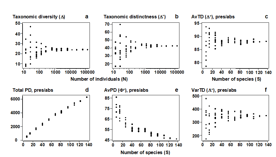
Fig. 17.2. Amoco-Cadiz oil spill {A}, pooled pre-impact data. a), b) Quantitative indices (y-axis): Average taxonomic diversity ($\Delta$) and distinctness ($\Delta ^ \ast$) for random subsets of fixed numbers of individuals (x-axis, logged), drawn randomly from the pooled sample, as in Fig. 17.1. c)–f) List-based (presence/absence) indices (y-axis): Average taxonomic distinctness ($\Delta ^ +$), total phylogenetic diversity (PD), average phylogenetic diversity ($\Phi ^ +$) and Variation in taxonomic distinctness ($\Lambda ^ +$), for random subsets of fixed numbers of species (x-axis) drawn from the full species list for the pooled sample. The sample-size independence of TD-based indices is clear, contrasting with PD and most standard diversity measures (Fig. 17.1).

^¶ The principle extends naturally to a phylogeny with continuously varying branch lengths and even, ultimately, to a molecular-based genetic distance between individuals (of the same or different species), see Clarke & Warwick (2001) , Fig. 1. And one of the interesting further developments is to apply the ideas of this chapter to a tree which reflects functional relationships among species, leading to functional diversity measures ( Somerfield, Clarke, Warwick et al. (2008) ).

^† In addition, there is a relationship between $\Delta$ and Simpson indices computed at higher taxonomic levels, see Shimatani (2001) . In effect, $\Delta$ is a (weighted) mean of Simpson at all taxonomic levels.

17.3 Examples: Ekofisk oil-field and Tees Bay soft-sediment macrobenthos

The earlier Fig. 14.4 demonstrated a change in the sediment macrofaunal communities around the Ekofisk oil-field {E}, out to a distance of about 3 km from the centre of drilling activity. This was only evident, however, from the multivariate (MDS and ANOSIM) analyses, not from univariate diversity measures such as Shannon H$^ \prime$, where reduced diversity was only apparent up to a few hundred metres from the centre (Fig. 17.3a). The implication is that the observed community change resulted in no overall loss of diversity but this is not the conclusion that would have been drawn from calculating the quantitative average taxonomic distinctness index, $\Delta ^ \ast$. Fig. 17.3b shows a clear linear trend of increase in $\Delta ^ \ast$ with (log) distance from the centre, the relationship only breaking down into a highly variable response for the strongly impacted sites, within 100m of the drilling activity.

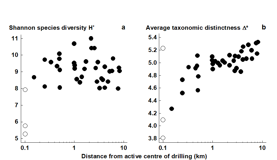
Fig. 17.3. Ekofisk macrobenthos {E}. a) Shannon diversity (H$^ \prime$) for the 39 sites (y-axis), plotted against distance from centre of drilling activity (x-axis, log scale). b) Quantitative average taxonomic distinctness $\Delta ^ \ast$ for the 39 sites, indicating a response trend not present for standard diversity indices.

A further example, from the coastal N Sea, is given by a time-series of macrobenthic samples, with data averaged over 6 locations in Tees Bay, UK, ({t}, Warwick, Ashman, Brown et al. (2002) ). Samples were taken in March and September for each of the years 1973 to 1996, and Fig. 17.4 shows the September inter-annual patterns for four (bio)diversity measures. Notable is the clear increase in Shannon diversity at around 1987/88 (Fig. 17.4b), coinciding with significant widescale changes in the N Sea planktonic system which have been reported elsewhere (e.g. Reid, Barges & Svendsen (2001) ). However, Shannon diversity is very influenced here by the high numbers of a single abundance dominant (Spiophanes bombyx), whose decline after 1987 led to greater equitability in the quantitative species diversity measures. A more far-reaching change, representative of what was happening to the community as a whole, is indicated by looking at the taxonomic relatedness statistics based only on presence/absence data. Use of simple species lists has the advantage here of ensuring that no one species can dominate the contributions to the index. Average taxonomic distinctness ($\Delta ^ +$) is seen to show a marked decline at about the time of this N Sea regime shift (Fig. 17.4c), indicating a biodiversity loss, a very different (and more robust) conclusion than that drawn from Shannon diversity.

Fig. 17.4. Tees macrobenthos {t}. (Bio)diversity indices for Tees Bay areas combined, from sediment samples in September each year, over the period 1973–96, straddling a major regime-shift in N Sea ecosystems, about 1987. a) Richness, S; b) Shannon, H$^ \prime$; c) Average taxonomic distinctness, $\Delta ^ +$, based on presence/absence and reflecting the mean taxonomic breadth of the species lists; d) Variation in taxonomic distinctness, $\Lambda ^ +$ (also pres/abs), reflecting unevenness in the taxonomic hierarchy.

17.4 Other relatedness measures

The remainder of this chapter deals only with data in the form of a species list for a locality (presence/absence data). There is a substantial literature on measures incorporating, primarily, phylogenetic relationships amongst species (see references in the review-type papers of Faith (1994) and Humphries, Williams & Vane-Wright (1995) ). The context is conservation biology, with the motivation being the selection of individual species, or sets of species (or reserves), with the highest conservation priority, based on the unique evolutionary history they represent, or their complementarity to existing well-conserved species (or reserves). Warwick & Clarke (2001) draw a potentially useful distinction of terminology between this individual species-focused conservation context and the use, as in this chapter, of relatedness information to monitor differences in community-wide patterns in relation to changing environmental conditions. They suggest that the term taxonomic/phylogenetic distinctiveness (of a species) is reserved for weights assigned to individual species, reflecting their priority for conservation; whereas taxonomic/phylogenetic distinctness (of a community) summarises features of the overall hierarchical structure of an assemblage (the spread, unevenness etc. of the classification tree).

Phylogenetic diversity (PD)

In the distinctiveness context, Vane-Wright, Humphries & Williams (1991) , Williams, Humphries & Vane-Wright (1991) and May (1990) introduced measures based only on the topology (‘elastic shape’) of a phylogenetic tree, appropriate when branch lengths are entirely unknown. Faith (1992) and Faith (1994) defined a phylogenetic diversity (PD) measure based on known branch lengths: PD is simply the cumulative branch length of the full tree. Whether this is thought of as representing the total evolutionary history, the genetic turnover or morphological richness, it is an appealingly simple statistic. Unfortunately, Fig. 17.5 demonstrates some of the disadvantages of using these measures in a distinctness context. The figure compares only samples (lists) with the same number of species (7), at four hierarchical levels (say, species within genera within families, all in one order), so that each step length is set to 33.3. Fig. 17.5b and c have the same tree topology, yet we should not consider them to have the same average (or total) distinctness, since each species is more taxonomically similar to its neighbours in b than c (reflected in $\Delta ^ +$ values of 33.3 and 66.6 respectively). Similarly, contrasting Fig. 17.5d and e, the total PD is clearly identical, the sum of all the branch lengths being 333 in both cases, but this does not reflect the more equitable distribution of species amongst higher taxa in d than e ($\Delta ^ +$ does, however, capture this intuitive element of biodiversity, with respective values of 52 and 43).

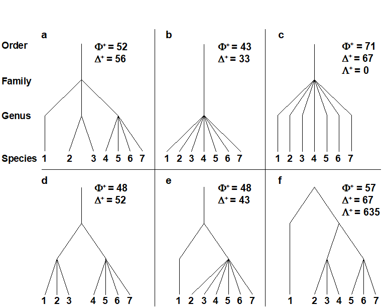
Fig. 17.5. a)-f) Example taxonomic hierarchies for presence/ absence data on 7 species (i.e. of fixed species richness), with 4 levels and 3 step lengths (thus each of 33.3, though the third step only comes into play for plot f). $\Phi ^ +$: average phylogenetic diversity,$\Delta ^ +$: average taxonomic distinctness, $\Lambda ^ +$: variation in TD. The plots show, inter alia: the expected ‘biodiversity’ decrease from a) to d) and e) to b) (in both $\Delta ^ +$ and $\Phi ^ +$), and from d) to e) (but only in $\Delta ^ +$, not in $\Phi ^ +$); unevenness of f) in relation to c), reflected in increased $\Lambda ^ +$ though unchanged $\Delta ^ +$.

Average PD

More importantly, there is another clear reason why phylogenetic diversity PD is unsuitable for monitoring purposes. Firstly, note that PD itself is a total rather than average property; as new species are added to the list it always increases. This makes PD highly dependent on species richness S and thus sampling effort, a demonstration of which can be seen in Fig. 17.2d (and the later Fig. 17.9a), a near straight line relationship of PD with S. This is to be expected, and a better equivalent to average taxonomic distinctness (AvTD, $\Delta ^ +$) would be average phylogenetic diversity (AvPD), defined as the ratio:

$$ \Phi ^ + = PD / S \tag{17.5} $$

This is a very intuitive summary of average distinctness, being the contribution that each species makes on average to the total tree length, but unfortunately it does not have the same lack of dependence on sampling effort that characterises $\Delta ^ +$. Fig. 17.2e (and the later Fig. 17.9b) show that its value decreases markedly as the number of species (S) increases, making it misleading to compare AvPD values across studies with differing levels of sampling effort.

‘Total’ versus ‘average’ measures

Note the distinction here between total and average distinctness measures. AvPD ($\Phi ^ +$) is the analogue of AvTD ($\Delta ^ +$), both being ways of measuring the average taxonomic breadth of an assemblage (a species list), for a given number of species. $\Delta ^ +$ will give the same value (on average) whatever that number of species; $\Phi ^ +$ will not. Total PD measures the total taxonomic breadth of the assemblage and has a direct analogue in total taxonomic distinctness:

$$ TTD = S \times \Delta ^ + = \sum _ i \left[ \left( \sum _ {j \ne i} \omega _ {ij} \right) / \left(S – 1 \right) \right] \tag{17.6} $$

Explained in words, this is the average taxonomic distance from species i to every other species, summed over all species, i = 1, 2, …, S. (Taking an average rather than a sum gets you back to AvTD, $\Delta ^ +$.) TTD may well be a useful measure of total taxonomic breadth of an assemblage, as a modification of species richness which allows for the species inter-relatedness, so that it would be possible, for example, for an assemblage of 20 closely-related species to be deemed less ‘rich’ than one of 10 distantly-related species. In general, however, like total PD, total TD will tend to track species richness rather closely, and will only therefore be useful for tightly controlled designs in which effort is identical for the samples being compared, or sampling is sufficiently exhaustive for the asymptote of the species-area curve to have been reached (i.e. comparison of censuses rather than samples).

Variation in TD

Finally, a comparison of Fig. 17.5c and f shows that the scope for extracting meaningful biodiversity indices (unrelated to richness) from simple species lists has not yet been exhausted. Average taxonomic distinctness is the same in both cases ($\Delta ^ + = 66.6$) but the tree constructions are very different, the former having consistent, intermediate taxonomic distances between pairs of species, in comparison with the latter’s disparate range of small and large values. This can be conveniently summarised in a further statistic, the variance of the taxonomic distances {$\omega_{ij}$} between each pair of species i and j, about their mean value $\Delta ^ +$:

$$ \Lambda ^ + = \left[ \sum \sum _ {i < j} ( \omega _ {ij} - \Delta ^ + ) ^ 2 \right] / \left[ S (S - 1)/2 \right] \tag{17.7} $$

termed the variation in taxonomic distinctness, VarTD. Its behaviour in a practical application will be examined later in the chapter^¶, but note for the moment that it, too, appears to have the desirable sampling property of (approximate) lack of dependence of its mean value on sampling effort (see Fig. 17.2f).

^¶ The PRIMER DIVERSE routine has options to compute the full range of relatedness-based biodiversity measures discussed in this chapter: $\Delta$, $\Delta ^ \ast$, $\Delta ^ +$, TTD, $\Lambda ^ +$, PD, $\Phi ^ +$, simultaneously for all the samples in a species matrix. It returns the values to a worksheet which can be displayed as Scatter Plots, Histograms, Draftsman Plots etc, analysed in a multivariate way (with the indices as the variables, page 8.7) or by conventional univariate tests, either in PERMANOVA on Euclidean distance matrices from single indices ( Anderson, Gorley & Clarke (2008) ) or exported to ANOVA software. These DIVERSE options require the availability of an aggregation file, detailing which species map to which genus, families etc, in exactly the same format needed for the Aggregate routine used to perform higher taxonomic level analyses in Chapter 10.

17.5 ‘Expected distinctness’ tests

Species master list

The construction of taxonomic distinctness indices from simple species lists makes it possible to address another of the ‘desirable features’ listed at the beginning of the chapter: there is a potential framework within which TD measures can be tested for departure from ‘expectation’. This envisages a master list or inventory of species, within defined taxonomic boundaries and encompassing the appropriate region/biogeographic area, from which the species found at one locality can be thought of as drawn. For example, the next illustration uses the full British faunal list of 395 free-living marine nematodes, updated from the keys of Platt & Warwick (1983) and Platt & Warwick (1988) . The species complement at any specific locality and/or historic period (e.g. putatively impacted areas such as Liverpool Bay or the Firth of Clyde) can be compared with this master list, to ask whether the observed subset of species represents the biodiversity expressed in the full species inventory. Clearly, such a comparison is impossible for species richness S, or total TD or PD, since the list at one location is automatically shorter than the master list. Also, comparison of S between different localities (or historic periods) is invalidated by the inevitable differences in sampling effort in constructing the lists for different places (or times). However, the key observation here ( Clarke & Warwick (1998b) ) is that average taxonomic distinctness ($\Delta ^ +$) of a randomly selected sublist does not differ, in mean value, from AvTD for the master list. So, localities that have attracted differing degrees of sampling effort are potentially directly comparable, with each other and with $\Delta ^ +$ for the full inventory. The latter is the ‘expected value’ for average distinctness from a defined faunal group, and reductions from this level, at one place or time, can potentially be interpreted as loss of biodiversity.

Testing framework

Furthermore, there is a natural testing framework for how large a decrease (or increase) from expectation needs to be, in order to be deemed statistically ‘significant’. For an observed set of m species at one location, sublists of size m are drawn at random from the master inventory, and their AvTD values computed. From, say, 999 such simulated sublists, a histogram can be constructed of the expected range of $\Delta ^ +$ values, for sublists of that size, against which the true $\Delta ^ +$ for that locality can be compared. If the observed $\Delta ^ +$ falls outside the central 95% of the simulated $\Delta ^ +$ values, it is considered to have departed significantly from expectation: a two-sided test is probably appropriate since departure could theoretically be in the direction of enhanced as well as reduced distinctness.

The next stage is to repeat the construction of these 95% probability intervals for a range of sublist sizes (m = 10, 15, 20, …) and plot the resulting upper and lower limits on a graph of $\Delta ^ +$ against m. When these limit points are connected across the range of m values, the effect is to produce a funnel plot (such as seen in Fig. 17.8). The real $\Delta ^ +$ values for a range of observational studies are now added to this plot, allowing simultaneous comparison to be made of distinctness values with each other and with the ‘expected’ limits.^¶

^¶ Histogram and funnel plots of the ‘expected’ spread of $\Delta ^ +$ values for a given subsample size (or size range), drawn from a master species list, are plotted in the PRIMER TAXDTEST routine, accessible when the active sheet is the aggregation file for the master list. An option is given to superimpose a real data value on the simulated histogram, or a set of real values on the funnel plot.

17.6 Example: UK free-living nematodes

Warwick & Clarke (1998) examined 14 species lists from a range of different habitats and impacted/undisturbed UK areas ({U}, Fig. 17.6), referring them to a 6-level classification of free-living, marine nematodes ( Lorenzen (1994) ), based on cladistic principles. The taxonomic groupings were: species, genus, family, suborder, order and subclass, all within one class, thus giving equal step lengths between adjacent taxonomic levels of 16.67 (species within different subclasses then being at a taxonomic distance of $\omega = 100$). The relatively comprehensive British master list (updated from Platt & Warwick (1983) , Platt & Warwick (1988) , Warwick, Platt & Somerfield (1998) ) consisted of 395 species, the individual area/ habitat sublists ranging in size from 27 to 164 species. They included two studies of the same (generally impacted) area, the Firth of Clyde, carried out by different workers and resulting in very disparate sublist sizes (53 and 112).

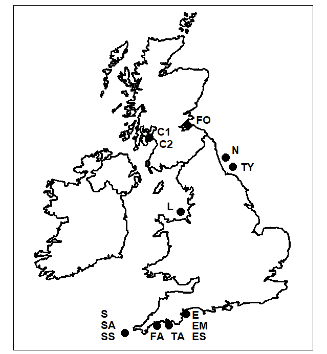
Fig. 17.6. UK regional study, free-living nematodes {U}. The location/habitat combinations for the 14 species sublists whose taxonomic distinctness structure is to be compared. Sublittoral offshore sediments at N: Northumberland ( Warwick & Buchanan (1970) ); TY: Tyne ( Somerfield, Gee & Widdicombe (1993) ); L: Liverpool Bay ( Somerfield, Rees & Warwick (1995) . Intertidal sand beaches at ES: Exe ( Warwick (1971) ); C1: Clyde ( Lambshead (1986) ); C2: Clyde ( Jayasree (1976) ); FO: Forth ( Jayasree (1976) ); SS: Scilly ( Warwick & Coles (1977) ). Estuarine intertidal mudflats at EM: Exe ( Warwick (1971) ); TA: Tamar ( Austen & Warwick (1989) ); FA: Fal ( Somerfield, Gee & Warwick (1994a) and Somerfield, Gee & Warwick (1994b) ). Algal habitats in SA: Scilly ( Gee & Warwick (1994a) and Gee & Warwick (1994b) ). Also mixed habitats at E: Exe, S: Scilly.

Histograms

Species richness levels of the 14 lists are clearly not comparable since sampling effort is unequal. However, the studies have been rationalised to a common taxonomy and AvTD values may be meaningfully compared. Fig. 17.7 contrasts two of the studies, which have similar-length species lists: sandy sites in the Exe estuary (ES, 122 species) and the Firth of Clyde (C1, 112 species). Fig. 17.7a displays the histogram of $\Delta ^ +$ values for 999 random subsamples of size m = 122, drawn from the full inventory of 395 species, and this is seen to be centred around the master AvTD of 78.7, with a (characteristic) left-skewness to the $\Delta ^ +$ distribution. The observed $\Delta ^ +$ of 79.1 for the Exe data falls very close to this mean, in the body of the distribution, and therefore suggests no evidence of reduced taxonomic distinctness. Fig. 17.7b shows the histogram of simulated $\Delta ^ +$ values in subsets of size m = 112, having (of course) the same mean $\Delta ^ +$ of 78.7 but, in contrast, the observed $\Delta ^ +$ of 74.1 for the Clyde data now falls well below its value for any of the randomly selected subsets, demonstrating a significantly reduced average distinctness.

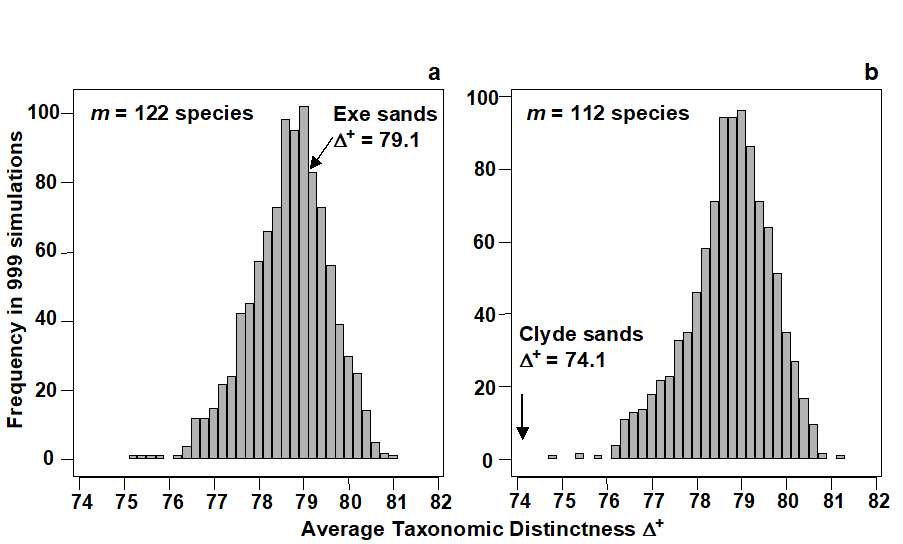
Fig. 17.7. UK regional study, free-living nematodes {U}. Histograms of simulated AvTD, from 999 sublists drawn randomly from a UK master list of 395 species. Sublist sizes of a) m=122, b) m=112, corresponding to the observed number of species in the Exe (ES) and Clyde (C1) surveys. True $\Delta ^ +$ also indicated: the Exe value is central but the null hypothesis that AvTD for the Clyde equates to that for the UK list as a whole is clearly rejected (p<0.001 or 0.1%)

Funnel plots

Fig. 17.8. UK regional study, free-living nematodes {U}. Funnel plot for simulated AvTD, as in Fig. 17.7, but for a range of sublist sizes m=10, 15, 20, …, 250 (x-axis). Crosses, and thick lines, indicate limits within which 95% of simulated $\Delta^+$ values lie; the thin line indicates mean $\Delta ^ +$ (the AvTD for the master list), which is not a function of m. Points are the true AvTD (y-axis) for the 14 location/habitat studies (see Fig. 17.6 for codes), plotted against their sublist size (x-axis).

Fig. 17.8 displays the funnel plot, catering for all sublist sizes. The simulated 95% probability limits are again based on 999 random selections for each of m = 10, 15, 20, …, 250 species from the 395. The mean $\Delta ^ +$ is constant for all m (at 78.7) but the limits become increasingly wide as the sample size decreases, reducing the likelihood of being able to detect a change in distinctness (i.e. reducing the power of the test). The probability limits also demonstrate the left-skewness of the $\Delta ^ +$ distribution about its mean throughout, though especially for low numbers of species. Superimposing the real $\Delta ^ +$ values for the 14 habitat/location combinations, five features are apparent:

The impacted areas of Clyde, Liverpool Bay, Fal and, to a lesser extent, Tamar, are all seen to have significantly reduced average distinctness, whereas pristine locations in the Exe and Scilly have $\Delta ^ +$ values close to that of the UK master list.
Unlike species richness (and in keeping with the ‘desirability criteria’ stated earlier), $\Delta^+$ does not appear to be strongly dependent on habitat type: Exe sand and mud habitats have very different numbers of species but rather centrally-placed distinctness; Scilly algal and sand habitats have near-identical $\Delta ^ +$ values. Warwick & Clarke (1998) also demonstrate a lack of habitat dependence in $\Delta ^ +$ from a survey of Chilean nematodes (data of W Wieser).
There is apparent monotonicity of response of the index to environmental degradation (also in keeping with another initial criterion). To date, there is no evidence of average taxonomic distinctness increasing in response to stress.
In spite of the widely differing lengths of their species lists, it is notable that the two Clyde studies (C1, C2) return rather similar (depressed) values for $\Delta ^ +$.
There is no evidence of any empirical relation in the ($\Delta ^ +$, S) scatter plot. We know from the sampling theory that the mechanics of calculating $\Delta ^ +$ does not lead to an intrinsic relationship between the two but that does not prevent there being an observed correlation; the latter would imply some genuine assemblage structuring which predisposed large communities to be more (or less) ‘averagely distinct’ than small communities. The lack of an intrinsic, mechanistic correlation greatly aids the search for such interesting observational relationships (see also the later discussion on AvTD, VarTD correlations). The same cannot be said for phylogenetic diversity, PD. Fig. 17.9a shows the expected near-linear relation between total PD and S for these meiofaunal studies (total TD and S would have given a similar picture) but, more significantly, Fig. 17.9b bears out the previous statements about the dependence also of average PD ($\Phi ^ +$) on S. This intrinsic relationship, shown by the declining curve for the expected value of $\Phi^+$ as a function of the number of species in the list, contrasts markedly with the constant mean line for $\Delta ^ +$ in Fig. 17.8. Nothing can therefore by read into an observed negative correlation of $\Phi ^ +$ and S in a practical study: such a relationship would be likely, as here, to be purely mechanistic, i.e. artefactual.

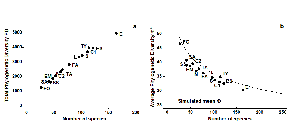
Fig. 17.9. UK regional study, free-living nematodes {U}. Scatter plots for the 14 location/habitat studies (Fig. 17.6) of: a) total PD, b) AvPD against list size m, the latter also showing the declining ‘expected’ mean $\Phi ^ +$ with m, simulated from sublists of the UK master list.

AvTD is therefore seen to possess many of the features listed at the beginning of the chapter as desirable in a biodiversity index – a function, in part, of its attractive mathematical sampling properties (for formal statistical results on unbiasedness and variance structure see Clarke & Warwick (1998b) and Clarke & Warwick (2001) ). Many questions remain, however – from theoretical issues of its dependence (or lack of it) on essentially arbitrary assumptions about relative weighting of step lengths through the taxonomic tree, to further practical demonstration of its performance (or lack of it) for other faunal groups and environmental impacts. The following example addresses these two questions in particular.

17.7 Example: N Europe groundfish surveys

An investigation of the taxonomic structure of demersal fish assemblages in the North Sea, English Channel and Irish Sea, motivated by concerns over the impacts of beam trawling, is reported by Rogers, Clarke & Reynolds (1999) . A total of 277 ICES quarter-rectangles were sampled for 93 species of groundfish {b}, by research vessels from different N European countries. Sampling effort per rectangle was not constant. For the purposes of display, quarter-rectangles were grouped into 9 larger sea-areas: 1–Bristol Channel, …, 9–Eastern Central N Sea (Fig. 17.10, see legend for area definitions).

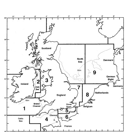
Fig. 17.10. Beam-trawl surveys, for groundfish, N Europe {b}. 277 rectangles from 9 sea areas. 1: Bristol Channel, 2: W Irish Sea, 3: E Irish Sea, 4: W Channel, 5: NE Channel, 6: SE Channel, 7: SW North Sea, 8: SE North Sea, 9: E Central North Sea.

There is a wealth of taxonomic detail to exploit in this case. The analysis uses a 14-level classification (Fig. 17.11), based on phylogenetic information, compiled by J.D. Reynolds (Univ E Anglia), primarily from Nelson (1994) and McEachran & Miyake (1990) . The distinctness structure of this master list, and its AvTD of $\Delta ^ + = 80.1$, for all groundfish species that could be reliably sampled and identified, becomes the standard against which the species lists from the various quarter-rectangles are assessed.

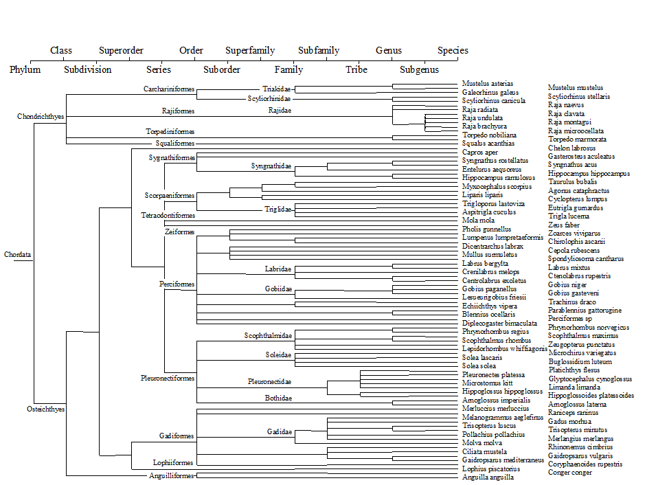
Fig. 17.11. Beam-trawl surveys, for groundfish, N Europe {b}. 14-level classification (phylogenetically-based) used for the construction of taxonomic distances between 93 demersal fish species, those that could be reliably sampled and identified for the 277 rectangles in this N European study.

Funnel plot

Fig. 17.12 displays the resulting funnel plot of the range of $\Delta ^ +$ values expected from sublists of size 5 to 35, repeating the mean, lower and upper limits in sub-plots of observed $\Delta ^ +$ values for the 9 sea areas. $\Delta ^ +$ is clearly seen to be reduced in some areas, particularly 6, 8 and 9, whilst remaining at ‘expected’ levels in others. Rogers, Clarke & Reynolds (1999) discuss possible explanations for this, noting the contribution made by the spatial pattern of elasmobranchs, a taxonomic group they argue may be particularly susceptible to disturbance by commercial trawling, because of their life history traits.

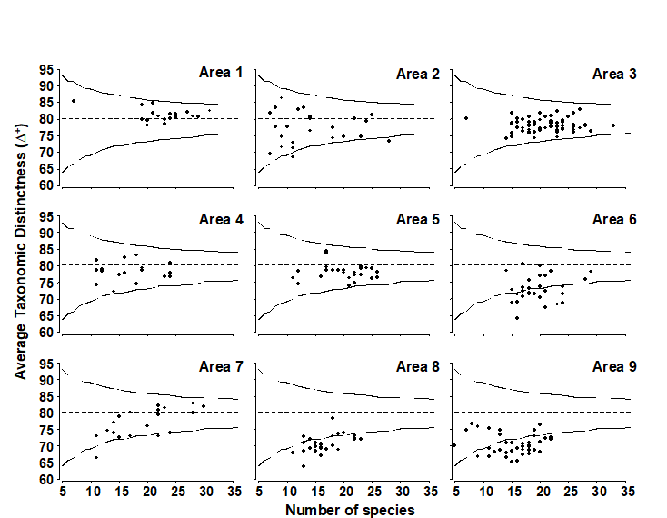
Fig. 17.12. Beam-trawl surveys, for groundfish, N Europe {b}. AvTD (presence/absence data) against observed number of species, in each of 274 rectangles, grouped into 9 sea areas (Fig. 17.10). Dashed line indicates mean of 5000 simulated sublists for each size m = 5, 6, 7, …, 35, confirming the theoretical unbiasedness and therefore comparability of $\Delta ^ +$ for widely differing degrees of sampling effort. Continuous lines denote 95% probability limits for $\Delta ^ +$ from a single sublist of specified size from the master list (of 93 species).

Weighting of step lengths

Many of the fine-scale phylogenetic groupings in Fig. 17.11 are utilised comparatively rarely (e.g. subgenera only within Raja, tribe only within the Pleuronectidae etc), and the standard assumption that all step lengths between taxonomic levels are given equal weight (7.69, in this case) may appear arbitrary. For example, if a new category is defined which is not actually used, then the resulting change in all the step lengths, in order to accommodate it, seems unwarranted. The natural alternative here is to make the step lengths proportional to the extent of group melding that takes place, larger steps corresponding to larger decreases in taxon richness. A null category would then add no additional step length. Table 17.1 shows the resulting taxonomic distances {$\omega ^ {(0)}$} between species connected at the differing levels, contrasted with the standard, equal-stepped, distances {$\omega$}. Obviously, both are standardised so that the largest distance in the tree (between species in the different classes Chondrichthyes and Osteichthyes) is set to 100.

Table 17.1. Beam-trawl surveys, for groundfish, N Europe {b}. The 13 taxonomic/phylogenetic categories (k) used in the groundfish study, the standard taxonomic distances {$\omega _ k$} and an alternative formulation {$\omega _ k ^ {(0)}$} based on taxon richness {s_k} at each level. $\omega_k$ (or $\omega _ k ^ {(0)}$) is the path length between species from different taxon group k but the same group k+1.

k	Taxon	s_k	$\omega _ k$	$\omega _ k ^ {(0)}$
1	Species	93	7.7	1.3
2	Sub-genus	89	15.4	6.9
3	Genus	72	23.1	8.9
4	Tribe	67	30.8	12.5
5	Sub-family	59	38.5	21.4
6	Family	41	46.2	22.9
7	Super-family	39	53.8	27.4
8	Sub-order	33	61.5	44.4
9	Order	14	69.2	54.9
10	Series	9	76.9	61.4
11	Super-order	7	84.6	65.6
12	Sub-division	6	92.3	85.3
13	Class	2	100.0	100.0

Fig. 17.13 demonstrates the minimal effect these revised weights have on the calculation of average taxonomic distinctness, $\Delta ^ +$ . It is a scatter plot of $\Delta ^ {+ (0)}$ (revised weights) against $\Delta ^ +$ (standard, equal-stepped, distances) for the 277 quarter-rectangle species lists. The relation is seen to be very tight, with only about 3 samples departing from near-linearity. (These are outliers of very low species richness – in one case as few as 2 species – and have been removed from Fig. 17.12.) Clearly, the relative values of $\Delta ^ +$ are robust in this case to the precise definition of the step-length weights, a reassuring conclusion which is also borne out for the UK nematode study {U}. For the data of Fig. 17.8, Clarke & Warwick (1999) consider the effects of various alternative step-length definitions, consistently increasing or decreasing the weights at higher taxonomic levels as well as weighting them by changes in taxon richness. The only alteration to the conclusions came from decreasing the step lengths at the higher (coarsest) taxonomic levels, especially suppressing the highest level altogether (so that species within different subclasses were considered no more taxonomically distant than those within different orders). The Scilly data sets then showed a clear change in their average distinctness in comparison with the other 11 $\Delta ^ +$ values.^¶

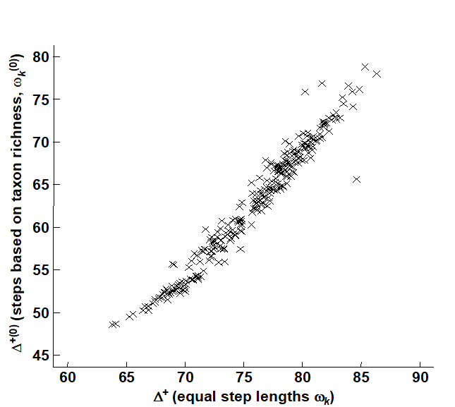
Fig. 17.13. Beam-trawl surveys, for groundfish, N Europe {g}. Comparison of observed $\Delta^+$, for each of 277 rectangles, between two weighting options for taxonomic distance between species: equal step-lengths between hierarchical levels (x-axis), and lengths proportional to change in taxonomic richness at that step (y-axis).

The unusual structure of the Scillies sublists is also exemplified, in a more elegant way, by considering not just average but variation in taxonomic distinctness.

^¶ Both the PRIMER DIVERSE and TAXDTEST routines allow such compression of taxonomic levels, either at the top or bottom of the tree (or both), and also permit automatic computation of step-length weights based on changes in taxon richness and, indeed, any user-specified weighting.

17.8 Variation in taxonomic distinctness, $\Lambda ^ +$

VarTD was defined in equation (17.7), as the variance of the taxonomic distances {$\omega _ {ij}$} between each pair of species i and j, about their mean distance $\Delta ^ +$. It has the potential to distinguish differences in taxonomic structure resulting, for example, in assemblages with some genera becoming highly species-rich whilst a range of other higher taxa are represented by only one (or a very few) species. In that case, average TD may be unchanged but variation in TD will be greatly increased, and Clarke & Warwick (2001) argue (on a sample of one!) that this might be expected to be characteristic of island fauna, such as that for the Isles of Scilly.

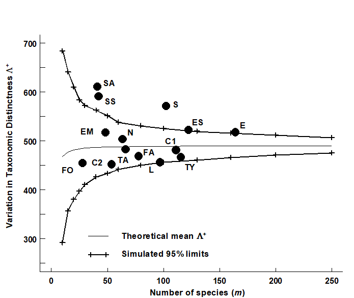
Fig. 17.14. UK regional study, free-living nematodes {U}. Funnel plot, as in Fig. 17.8, but for simulated VarTD ($\Lambda ^ +$), against sublist sizes m=10, 15, 20, …, 250 (x-axis), drawn from the 395-species master list. Thin line denotes the theoretical (and simulated) mean $\Lambda ^ +$, which is no longer entirely constant, declining very slightly for small values of m. The bias is clearly negligible, however, showing that (like $\Delta ^ +$) $\Lambda ^ +$ is comparable across studies with differing sampling effort (as here). Superimposed observed $\Lambda ^ +$ values for the 14 location/habitat combinations (Fig. 17.6) show a significantly larger than expected VarTD for the Scilly datasets.

For the UK nematode study {U}, Fig. 17.14 displays the funnel plot for VarTD ($\Lambda ^ +$) which is the companion to Fig. 17.8 (for AvTD, $\Delta ^ +$). It is constructed in the same way, by many random selections of sublists of a fixed size m from the UK master list of 395 nematode species, and recomputation of $\Lambda ^ +$ for each subset. The resulting histograms are typically more symmetric than for $\Delta ^ +$, as seen by the 95% probability limits for ‘expected’ $\Lambda ^ +$ values, across the full range of sublist sizes: m = 10, 15, 20, 25, …, shown in Fig. 17.14. Three features are noteworthy:

The simulated mean $\Lambda ^ +$ (thin line in Fig. 17.14) is again largely independent of sublist size, only declining slightly for very short lists (and the slight bias is dwarfed by the large uncertainty at these low sizes). Clarke & Warwick (2001) derive an exact formula for the sampling bias of $\Lambda ^ +$ and show, generally, that it will be negligible. This again has important practical implications because it allows $\Lambda ^ +$ to be meaningfully compared across (historic) studies in which sampling effort is uncontrolled.
The various UK habitat/location combinations all fall within ‘expected’ ranges, with the interesting exception of the Scilly data sets. These have significantly higher VarTD values, as discussed above.
$\Lambda ^ +$ therefore appears to be extracting independent information, separately interpretable from $\Delta ^ +$, about the taxonomic structure of individual data sets. This assertion is testable by a bivariate approach.

17.9 Joint (AvTD, VarTD) analyses

The histogram and funnel plots of Figs. 17.7 and 17.8 are univariate analyses, concentrating on only one index at a time. Also possible is a bivariate approach in which ($\Delta ^ +$, $\Lambda ^ +$) values are considered jointly, both in respect of the observed outcomes from real data sets and their expected values under subsampling from a master species inventory. Fig. 17.15 shows the results of a large number of random selections of m = 100 species from the 395 in the UK nematode list {U}; each selection gives rise to an (AvTD, VarTD) pair and these are graphed in a scatter plot (Fig. 17.15a). Their spread defines the ‘expected’ region (rather than range) of distinctness behaviour, for a sublist of 100 species. Superimposed on the same plot are the observed ($\Delta ^ +$, $\Lambda ^ +$) pairs for three of the studies with list sizes of about that order: all three (Clyde, Liverpool Bay and Scilly) are seen to fall outside the expected structure, though in different ways, as previously discussed.

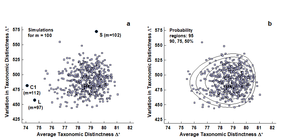
Fig. 17.15. UK regional study, free-living nematodes {U}. a) Scatter plot of (AvTD, VarTD) pairs from random selections of m = 100 species from the UK nematode list of 395; also superimposed are three observed points: Clyde (C1), Liverpool Bay (L) and Scilly (S), all falling outside ‘expectation’. b) Probability contours (back-transformed ellipses) containing approximately 95, 90, 75 and 50% of the simulated values. Both plots are based on 1000 simulations though only 500 points are displayed, for clarity.

‘Ellipse’ plots

It aids interpretation to construct the bivariate equivalent of the univariate 95% probability limits in the histogram or funnel plots, namely a 95% probability region, within which (approximately) 95% of the simulated values fall. An adequate description here is provided by the ellipse from a fitted bivariate normal distribution to separately transformed scales for $\Delta ^ +$ and $\Lambda ^ +$.

AvTD in particular needs a reverse power transform to eliminate the left-skewness though, as previously noted, any transformation of VarTD can be relatively mild, if needed at all. Clarke & Warwick (2001) discuss the fitting procedure in detail^¶ and Fig. 17.15b shows its success in generating convincing probability contours, containing very close to the nominal levels of 50, 75, 90 and 95% of simulated data points. In the normal convention, the ‘expected region’ is taken as the outer (95%) contour, which is an ellipse on the transformed scales, though typically ‘egg-shaped’ when back-transformed to the original ($\Delta ^ +$, $\Lambda ^ +$) plot.

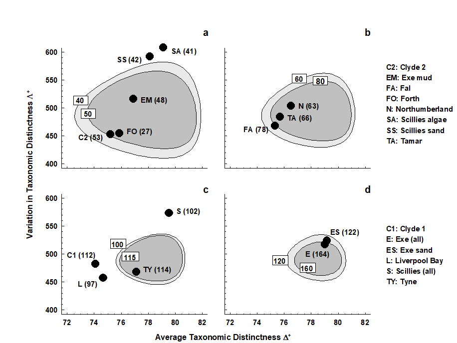
Fig. 17.16. UK regional study, free-living nematodes {U}. ‘Ellipse’ plots of 95% probability regions for (AvTD, VarTD) pairs, as for Fig. 17.15 but for a range of sublist sizes: a) m = 40, 50; b) m = 60, 80; c) m = 100, 115; d) m = 120, 160. The observed ($\Delta ^ +$, $\Lambda ^ +$) values for the 14 location/habitat studies are superimposed on the appropriate plot for their particular species list size (given in brackets). As seen in the separate funnel plots (Figs. 17.8 and 17.14), Clyde, Liverpool Bay, Fal (borderline) and all the Isles of Scilly data sets depart significantly from expectation.

A different region needs to be constructed for each sublist size or, in practice, for a range of m values, straddling the observed sizes. It may improve clarity to plot the regions in groups of two or three, as in Fig. 17.16. The conclusions are largely unchanged here, perhaps querying the need for a bivariate approach. However, there are at least three advantages to this:

A bivariate test naturally compensates for repeated testing which is inherent in separate univariate tests.
The ‘failure to reject’ region of the null hypothesis, inside the simulated 95% probability contour, is not rectangular, as it would be for two separate tests. This opens the possibility for other faunal groups, where simulated $\Delta ^ +$ and $\Lambda ^ +$ values may be negatively correlated (as appears to happen for components of the macrobenthos, Clarke & Warwick (2001) ), that significance could follow from the combination of moderately low AvTD and VarTD values, where neither of them on their own would indicate rejection.
It aids interpretation of spatial biodiversity patterns to know whether there is any intrinsic, artefactual correlation to be expected between the two indices, resulting from the fact that they are both calculated from the same set of data. Here, Fig. 17.15 shows emphatically that no such internal correlation is to be expected (though, as just commented, the independence of $\Delta ^ +$ and $\Lambda ^ +$ is not a universal result, and needs to be examined by simulation for each new master list). Yet the empirical correlation between $\Delta ^ +$ and $\Lambda ^ +$ for the 14 studies is not zero but large and positive (Fig. 17.17). This implies a genuine correlation from location to location in these two assemblage features, which it is legitimate to interpret. The suggestion ( Clarke & Warwick (2001) ) is that pollution may be connected with a loss both of the normal wide spread of higher taxa (reduced $\Delta ^ +$), and that the higher taxa lost are those with a simple subsidiary structure, represented only by one or two species, genera or families, leaving a more balanced tree (reduced $\Lambda ^ +$).

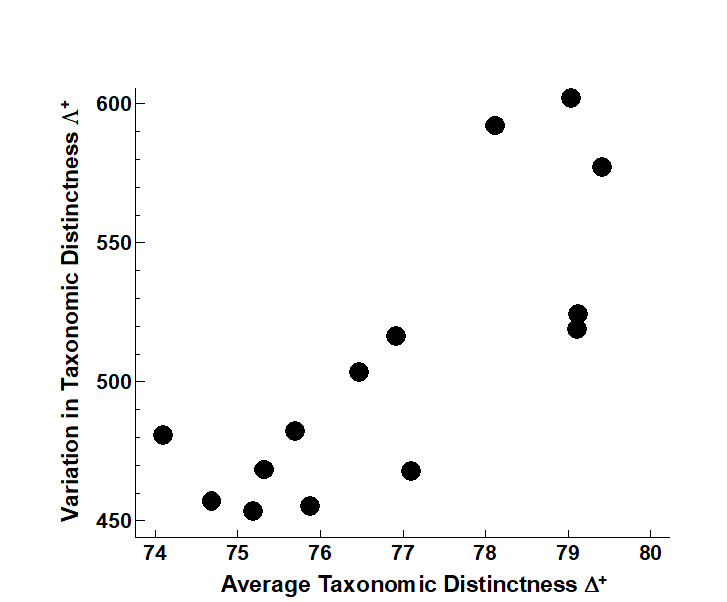
Fig. 17.17. UK regional study, free-living nematodes {U}. Simple scatter plot of observed (AvTD, VarTD) values for the 14 location/ habitat studies, showing the strongly positive empirical correlation (Pearson r = 0.79), which persists even if the three Scilly values are excluded (r = 0.75).

^¶ Accomplished by the PRIMER TAXDTEST routine, which automatically carries out the simulations and transformation/fitting of bivariate probability regions to obtain (transformed) ‘ellipse’ plots, for specified sublist sizes, on which real data pairs ($\Delta ^ +$, $\Lambda ^ +$) may be superimposed. Another variation introduced into TAXDTEST in later versions of PRIMER is to generate the model histograms, funnels etc for the ‘expected’ AvTD, VarTD not by assembling species by simple random picks from the master list, but by selecting species proportionally to their frequency of occurrence in a master data matrix (which will often be just the set of all samples in the study) – it can be argued that this provides a more realistic null hypothesis against which to compare the observed relatedness. The mean AvTD line is no longer quite independent of S (though dependence is weak) but funnels can be generated in just the same way – they may move slightly up or down the y axis, but again this modelling in no way changes the observed indices.

17.10 Concluding remarks on taxonomic distinctness

Early applications of taxonomic distinctness ideas in marine science can be found in Hall & Greenstreet (1998) for demersal fish, Piepenburg, Voss & Gutt (1997) for starfish and brittle-stars in polar regions, Price, Keeling & O’Callaghan (1999) for starfish in the Atlantic, and Woodd-Walker, Ward & Clarke (2002) for a latitudinal study of pelagic copepods. An early non-marine example is the work of Shimatani (2001) for forest stands. Over the last decade the index has become very widely used and cited. A bivariate example is given by Warwick & Light (2002) who use ‘ellipse’ plots of expected ($\Delta ^ +$, $\Lambda ^ +$) values, from live faunal records of the Isles of Scilly, to examine whether easily sampled bivalve and gastropod ‘death assemblages’ could be considered representative of the taxonomic distinctness structure of the live fauna.

Too much should not be claimed for these methods. It is surprising that anything sensible can be said about diversity at all, for data consisting simply of species presences, and arising from unknown or uncontrolled sampling effort (which usually renders it impossible to read anything into the relative size of these lists). Yet, much of the later part of this chapter suggests that not only can we find one index (AvTD) which is comparable across such studies, capturing an intuitive sense of biodiversity, but we can also find a second one (VarTD), with equally good statistical properties, and which may (sometimes at least) capture a near independent attribute of biodiversity structure.

Nonetheless, it is clear that controlled sampling designs, carried out in a strictly uniform way across different spatial, temporal or experimental conditions, must provide additional, meaningful, comparative diversity information (on richness, primarily) that $\Delta ^ +$ and $\Lambda ^ +$ are designed to ignore. Even here, though, concepts of taxonomic relatedness can expand the relevance of richness indices: rather than use S, or one of its variants (see Chapter 8), total taxonomic distinctness (TTD) or total phylogenetic diversity (PD), see page 17.4, capture the richness of an assemblage in terms of its number of species and whether they are closely or distantly related.

Sensitivity and robustness

Returning to the quantitative form $\Delta^*$, the Ekofisk oilfield study suggested that such relatedness measures may have a greater sensitivity to disturbance events than is seen with species-level richness or evenness indices ( Warwick & Clarke (1995a) and Warwick & Clarke (1995b) ). This suggestion was not borne out by subsequent oil-field studies ( Somerfield, Olsgard & Carr (1997) ), particularly where the impact was less sustained, the data collection at a less extensive level and hence the gradients more subtly entwined with natural variability. But it would be a mistake to claim sensitivity as a rationale for this approach: there is much empirical evidence that the best way of detecting subtle community shifts arising from environmental impacts is not through univariate indices at all, but by non-parametric multivariate display and testing (Chapter 14). The difficulty with the multivariate techniques is that, since they match precise species identities through the construction of similarity coefficients, they can be sensitive to wide scale differences in habitat type, geographic location (and thus species pool) etc.

Though independent of particular species identities, many of the traditional univariate indices have their own sensitivities, to habitat type, dominant species and sampling effort differences, as we have discussed. The general point here is that robustness (to sampling details) and sensitivity (to impact) are usually conflicting criteria. What is properly claimed for average taxonomic distinctness is not sensitivity but:

a) relevance – it is a genuine reflection of biodiversity loss, gain, or neither (rather than recording simply a change of assemblage composition), and one that appears to respond in a monotonic way to impact;

b) robustness – it can be meaningfully compared across studies from widely separated locations, with few (or even no) species in common, from different habitats, using data in presence/absence form (and thus not sensitive to dominant species), and with different sampling effort. This makes its natural use the comparison of regional/global studies and/or historic data sets, and it is no surprise to find that many of the citing papers address such questions.

Taxonomic artefacts

A natural question is the extent to which relatedness indices are subject to taxonomic artefacts. Linnean hierarchies can be inconsistent in the way they define taxonomic units across different phyla, for example. This concern can be addressed on a number of levels. As suggested earlier, the concept of mutual distinctness of a set of species is not constrained to a Linnean classification. The natural metric may be one of genetic distance (e.g. Nei (1996) ) or that from a soundly-based phylogeny combining molecular approaches with more traditional morphology. The Linnean classification clearly gives a discrete approximation to a more continuous distinctness measure, and this is why it is important to establish that the precise weightings given to the step lengths between taxonomic levels are not critical to the relative values that the index takes, across the studies being compared. Nonetheless, it is a legitimate concern that a cross-phyletic distinctness analysis could represent a simple shift in the balance of two major phyla as a decrease in biodiversity, not because the phylum whose presences are increasing is genuinely less (phylogenetically) diverse but because its taxonomic sub-units have been arbitrarily set at a lower level. Such taxonomic artefacts can be examined by computing the (AvTD, VarTD) structure across different phyla in a standard species catalogue, and Warwick & Somerfield (2008) show that the 4 major marine phyla do not suffer badly from this problem, though rare phyla with few species do have substantially lower AvTD. The pragmatic approach, as here, is to work within a well-characterised, taxonomically coherent group.

Master species list

Concerns about the precise definition of the master list (e.g. its biogeographic range or habitat specificity) also naturally arise. Note, however, that the existence of such a wide-scale inventory is not a central requirement, more of a secondary refinement. It is not used in constructing and contrasting the values of $\Delta ^ +$ for individual samples, and only features in two ways in these analyses:

In the funnel plots (Figs. 17.8, 17.12, 17.14), location of the points does not require a master species list, the latter being used only to display the background reference of the mean value and limits that would be expected for samples drawn at random from such an inventory. In Fig. 17.12, in fact, the limits are not even that relevant since they apply to single samples rather than, for example, to the mean of the tens of samples plotted for each sea area. The most useful plot for interpretation here is simply a standard means plot of the observed mean $\Delta ^ +$ and its 95% confidence interval, calculated from the replicates for each sea area (see Rogers, Clarke & Reynolds (1999) and Warwick & Clarke (2001) ).
In Table 17.1 and Fig. 17.3, the master species list is employed to calculate step lengths in a revised form of $\Delta ^ +$ – weighting by taxon richness at the different hierarchical levels. The existence of a master inventory makes this procedure more appealing, since if the taxon richness weighting was determined only by the samples to hand, the index would need to be adjusted as each new sample (containing further species) was added. The message of this chapter, however, is that the complication of adjusting weights in $\Delta ^ +$ for differences in taxon richness is unnecessary. Constant step lengths appear to be adequate.

The inventory is therefore only used for setting a background context, the theoretical mean and funnel limits. Various lists could sensibly be employed: global, local geographic, biogeographic provinces, or simply the combined species list of all the studies being analysed. The addition of a small number of newly-discovered species to the master inventory is unlikely to have a detectable effect on the overall mean and funnel for $\Delta ^ +$. If these are located in the taxonomic tree at random with respect to the existing taxa (rather than all belonging to the same high or low order group) they will have little or no effect on the theoretical mean $\Delta ^ +$. This, of course, is one of the advantages of using an index of average rather than total taxonomic distinctness.

It also makes clear what the limitations are to the validity of $\Delta ^ +$ comparisons. Whilst many marine community studies seem to consist of the low-level (species or genera) identifications which are necessary for meaningful computation of $\Delta ^ +$, there are always some taxa that cannot be identified to this level. There is no real difficulty here, since $\Delta ^ +$ is always used in a relative manner, provided these taxa are treated in the same way in all samples (e.g. treated as a single species in a single genus, single family, etc., of that higher taxon). The ability to impose taxonomic consistency is clearly an important caveat on the use of taxonomic distinctness for historic or widely-sourced data sets. Where such conditions can be met, however, we believe that these and similar formulations based on species relatedness, have a useful role in biodiversity assessment of biogeographic pattern and widescale change.

17.11 Taxonomic dissimilarity

A natural extension of the ideas of this chapter is from $\alpha$- or ‘spot’ diversity indices to $\beta$- or ‘turn-over’ diversity. The latter are essentially based on measures of dissimilarity between pairs of samples, the starting point for most of the methods of this manual. It is intriguing to ask whether there are natural analogues of some of the widely-used ‘biological’ dissimilarity coefficients, such as Sørensen (Bray-Curtis on presence/absence data, equation 2.7) or Kulczynski (P/A, equation 2.8), which exploit the taxonomic, phylogenetic or genetic relatedness of the species making up the pair of samples being compared. Thus two samples would be considered highly similar if they contain the same species, or closely related ones, and highly dissimilar if most of the species in one sample have no near relations in the other sample.

In fact, Clarke & Warwick (1998a) first defined a taxonomic mapping similarity between two species lists, in order to examine the taxonomic relatedness of the species sets successively ‘peeled’ from the full list, in a structural redundancy analysis of influential groups of species (the M statistic of Chapter 16, Table 16.2). This turns out to be the natural extension of Kulczynski dissimilarity and (to be consistent with our use in Chapter 17 of u.c. Greek characters for taxonomic relatedness measures) it is denoted here by $\Theta ^ +$. Izsak & Price (2001) used a slightly different form of coefficient, which proves to be the extension of the Sørensen coefficient, denoted here by $\Gamma ^ +$. Before defining these coefficients, however, it is desirable to state the potential benefits of such a taxonomic dissimilarity measure:

a) samples from different biogeographic regions do not lend themselves to conventional clustering or MDS ordination analyses using Sørensen (Bray-Curtis) or other traditional similarity coefficients. This is because few species may be shared between samples from different parts of the world. In extreme cases, there may be no species in common among any of the samples and all Bray-Curtis dissimilarities will be 100, leaving no possibility for a dendrogram or ordination plot. A taxonomic dissimilarity measure, however, takes into account not just whether the second sample has matching species to the first sample but, if it does not, whether there are closely related species in the second sample to all those found in the first sample (and vice-versa). Two lists with no species in common therefore have a defined dissimilarity, measuring whether they contain distantly or closely related species, and meaningful MDS plots ensue.

b) standard similarity measures will, inevitably, be susceptible to variation in taxonomic expertise or (in the case of time series) revisions in taxonomic definition, across the samples being compared. For example, suppose at some point in a time series, an increase in taxonomic expertise results in what was previously identified as a single taxon being noted as two separate species. The data should, of course, be subsequently rationalised to the lowest common denominator of taxonomic identification over the full series, but if this is not done, an ordination will have a tendency to display some artefactual signal of ‘community change’ at this point (one species has disappeared and two new ones have appeared). A single occurrence of this sort will not have much effect – one of the advantages of similarities based on presence/absence data is that they draw only a little information from each species – but if taxonomic inconsistency is rampant, misleading ordinations could result. Taxonomic dissimilarity would, however, be more robust to species being split in this way. The later samples do not appear to have the same taxon as the earlier samples, but they have one (or two) species which are very closely related to it (the same genus), hence retain high contributions to similarity from that species.

c) it might be hoped that the desirable sampling properties of taxonomic distinctness indices such as $\Delta ^ +$ and $\Lambda ^ +$, in particular their robustness to variable sampling effort across the samples, would carry over to taxonomic dissimilarity measures.

Taxonomic dissimilarity definition

As in Table 16.2, the distance through the taxonomic, (or phylogenetic/genetic) hierarchy, from every species in the first sample (A) to its nearest relation in the second sample (B), is recorded. These are totalled, as are the distances between species in sample B and their nearest neighbours in sample A, see the example in Fig. 17.18. These two totals are not the same, in general, and the way they are converted to an average taxonomic distance between the two samples defines the difference between $\Gamma ^ +$ and $\Theta ^ +$. Formally, if $\omega _ {ij}$ is the path length between species i and j, and there are $s _ A$ and $s _ B$ species in samples A and B, then:

$$\Gamma ^ + = 100 \times \left( \sum _ {i \in A} \min _ {j \in B} ( \omega _ {ij} ) + \sum _ {j \in B} \min _ {i \in A} ( \omega _ {ji}) \right) \big/ (s _ A + s _ B)$$ $$\Theta ^ + = 100 \times \frac{1}{2} \left( \frac{ \sum _ {i \in A} \min _ {j \in B} ( \omega _ {ij} )}{s _A} + \frac{ \sum _ {j \in B} \min _ {i \in A} ( \omega _ {ji})}{s _B} \right) \tag{17.8}$$

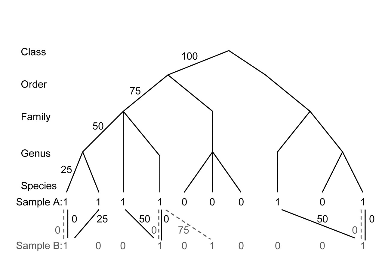
Fig. 17.18. For presence/absences from two hypothetical samples (A with 6 species, B with four), distances through the tree from each species in A to its nearest neighbour in B (black, continuous join) and vice-versa (grey, dashed join).

In words, $\Gamma ^ +$ is the average path length to the nearest relation in the opposite sample^¶, i.e. a simple average of all the path lengths shown in Fig. 17.18. Thus:

$$\Gamma ^ + = [(0+25+50+0+50+0)+(0+0+75+0)]/(6+4) = 20.0 $$

whereas $\Theta ^ +$ is a simple mean of the separate averages in the two directions: A to B, then B to A. Thus:

$$\Theta ^ + = [(125/6) + (75/4)]/2 = 19.8 $$

Clearly, the two measures give identical answers if the number of species is the same in the two samples, and they cannot give very different dissimilarities unless the richness is highly unbalanced. This is precisely as found for the relationship between the Bray-Curtis and Kulczynski measures on P/A data; they cannot give a different ordination plot unless species numbers are very variable. The relation of these standard coefficients to $\Gamma ^ +$ and $\Theta ^ +$ is readily seen: imagine flattening the taxonomic hierarchy to just two levels, species and genus, with all species in the same genus, so that different species are always 100 units apart. The branch length between a species in sample A and its nearest neighbour in sample B is either 0 (the same species is in sample B) or 100 (that species is not found in sample B). In that case:

$$\Gamma ^ + = (300 + 100)/(6+4) = 40.0 \equiv B ^ + $$ $$ \Theta ^ + = (300/6 + 100/4)/2 = 37.5 \equiv K ^ + \tag{17.8}$$

where $B ^ +$ and $K ^ +$ denote Bray-Curtis and Kulczynski dissimilarity for P/A data, respectively. The truth of this identity can be seen from their general definitions (see equations 2.7 and 2.8 for the similarity forms):

$$ B ^ + = (100 b + 100 c)/[(a + b) + (a + c)] $$ $$ K ^ + = [(100 b)/(a + b) + (100 c) / (a + c)]/2 \tag{17.9} $$

where b is the number of species present in sample A but not sample B, c is the number present in B but not A, and a is the number present in both. Clearly, 100b is the total of the (a+b) path lengths from A to B, and 100c the total of the (a+c) path lengths from B to A.

Taxonomic dissimilarity, $\Gamma ^ +$, is therefore a natural generalisation of the Sørensen coefficient, adding a more graded hierarchy on top of standard Bray-Curtis (instead of matching ‘hits’ and ‘misses’ there are now ‘near hits’ and ‘far misses’). In some ways, this is analogous to the relationship shown earlier, between Simpson diversity ($\Delta ^ \circ$) and taxonomic diversity ($\Delta$), and it has two likely consequences:

ordinations based on $\Gamma ^ +$ will bear an evolutionary, rather than revolutionary, relationship to those based on P/A Bray-Curtis^†; when there are many direct species matches $\Gamma ^ +$ may tend to track B$^ +$ rather closely.
$\Gamma ^ +$ will tend to carry across the sampling properties of B$^ +$; it is well-known that Bray-Curtis (and indeed, all widely-used dissimilarity coefficients) are susceptible to bias from variations in sampling effort. It is axiomatic in multivariate analysis that similarities be calculated between samples which are either rigidly controlled to represent the same degree of sampling effort, or in the case of non-quantitative sampling, samples are large enough for richness to be near the asymptote of the species -area curve (this is very difficult to arrange in most practical contexts!) Otherwise, it is inevitable that samples of smaller extent will contain fewer species and thus similarities calculated with larger samples will be lower, even when true assemblages are the same. Theory shows that, indeed, $\Gamma ^ +$ and $\Theta ^ +$ (along with B$^ +$, K$ ^ +$, $\Phi ^ +$) are not independent of sampling effort, so the third of our hoped-for properties for taxonomic dissimilarity – that it would carry across the nice statistical properties of taxonomic distinctness measures $\Delta ^ +$ and $\Lambda ^ +$ – is not borne out^§.

The other two potential advantages of taxonomic dissimilarity, given above, do stand up to practical examination. One of us (PJS), in the description of these taxonomic dissimilarity measures in Clarke, Somerfield & Chapman (2006) , gives the following two examples.

^¶ $\Gamma ^ +$ is the taxonomic distance, ‘TD’, of Izsak & Price (2001) (not to be confused with the AvTD and TTD of this chapter, which are diversity indices not dissimilarities!), except that the longest path length in their taxonomic trees is not scaled to a fixed number, such as 100 or 1, so they rescale it in similarity form, denoted $\Delta _s$.

^† It is tempting to define, by analogy with equations (17.1) to (17.3), a further coefficient, the ratio $\Phi ^ + = \Gamma ^ + / B ^ +$, which reflects more purely the relatedness dissimilarity, removing the Bray-Curtis component in $\Gamma ^ +$, coming from direct species matches. In fact, $\Phi ^ +$ is simply the average of the minimum distance from each species to its nearest relation in the other sample, calculated only for the ‘b+c’ species which do not have a direct match. It is thus independent of ‘a’ (number of matches) as well as ‘d’ of course (number of joint absences). Limited practical experience, however, suggests that $\Phi ^ +$ tends to ‘throw the baby out with the bathwater’ and leads to uninterpretably ‘noisy’ ordination plots.

^§ Note, however, that Izsak & Price (2001) provide some limited simulation evidence for $\Gamma ^ +$ being less biased by uneven sampling effort than one of the other standard P/A indices, Jaccard, equation (2.6). This suggests that the comparison with Sørensen – the more natural comparator, given the above discussion – would also indicate some advantage for the taxonomic dissimilarity measure (Jaccard and Sørensen are quite closely linked, in fact monotonically related, so they produce identical non-metric MDS plots for example).

17.12 Examples

Example: Island fish species lists

Fish species lists extracted from FishBase for a selection of 26 world island groups {i} were slimmed down to leave only species that are ‘endemic’ to the total list, in the sense of being found at only one of these 26 locations. This is an artificial construction, clearly, but it makes the point that the presence/absence matrix which results could never be input to species-level multivariate analysis because all locations then have no species in common, i.e. are 100% dissimilar to each other, and the Bray-Curtis resemblance matrix is uninformative. However, if the taxonomic dissimilarity $\Gamma ^ +$ is calculated for this data, the MDS ordination of Fig. 17.19 is obtained.

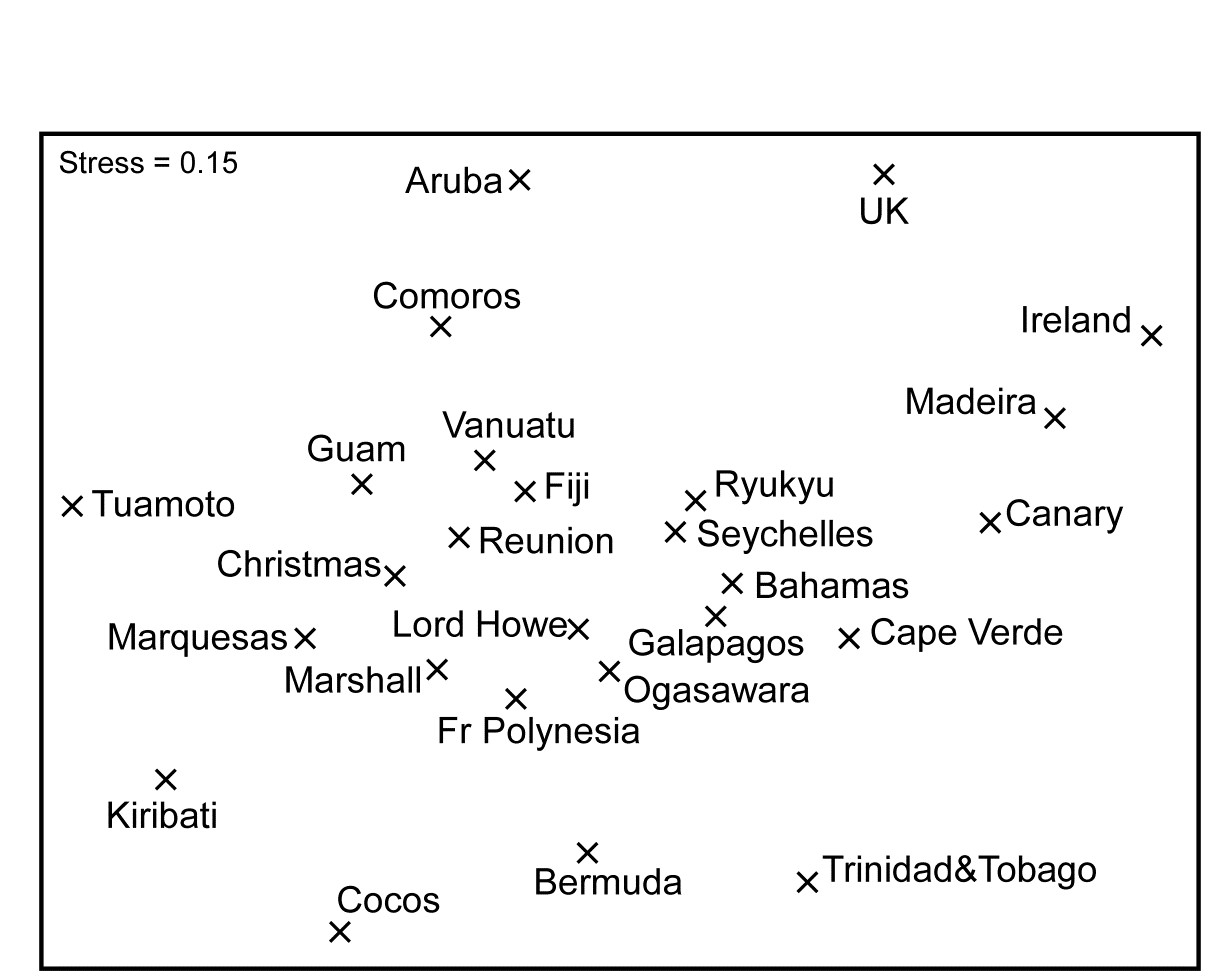
Fig. 17.19. Island group fish species {i}. nMDS ordination from presence/absence data on (pseudo-)endemic species found at 26 island groups, using taxonomic dissimilarity $\Gamma ^ +$.

Whilst this has reasonably high stress, a somewhat interpretable pattern of biogeographic relationships among the island groups is evident.

Example: Valhall oilfield macrofauna

This is another oilfield study, similar to the Ekofisk data ({E}), in which sediment samples are taken at one of five distance groups from the oilfield centre (0.5, 1, 2, 4 and 6 km), in a cross-hair design, and the macrobenthos examined through the time-course of operation of the field (data discussed by Olsgard, Somerfield & Carr (1997) , {V}). The data used here is of 20 samples taken in two years, 1988 and 1991, and the questions of interest concern not just whether a gradient of change exists in the community moving away from the field (which is clear) but whether this gradient is longer – a more accentuated change – in the later year.

After reduction to presence/absence and computation of Bray-Curtis dissimilarity (Sørensen, in effect, see equation 2.7) the nMDS of data from both years in a single ordination is shown in Fig. 17.20a. Whilst it is clear that there is a gradient of change away from the field in a parallel direction for the two years, the most obvious feature is the apparently large change in the community between 1988 and 1991 at all distances, and this certainly makes it difficult to gauge the size of relative changes along the two gradients. This gulf between the two years, e.g. even in the background community at 6km distant from the field, would not be expected at all, and is quite clearly an artefact. It does not take long to realise that the problem was that in 1988 (presumably with less-skilled contractors) the species were not identified with the same degree of discrimination: many species identified only as A in the earlier year had been split into species A and B (or even A, B, C, ..) in the later year, leading to an apparent major increase in species richness! Such an (artefactual) change in the data – an apparent influx of a large number of ‘new’ species – is certain to lead to the wide division of the two years in the MDS. The best solution, of course, is always to work with data at the lowest common denominator of identification: loss of precision in failing to split ‘difficult’ species is usually inconsequential in comparison to artefacts that arise from using inconsistent identification.

Such identification issues can be less obvious than in this case, of course: they may occur infrequently and balance out in terms of numbers of species recorded.

Fig. 17.20. Valhall oilfield macrofauna {V}. nMDS ordinations of macrobenthos from 20 sites in 5 distance groups from the oilfield centre, sampled in 1988 and 1991, using presence/absence data and: a) Bray-Curtis (Sørensen); b) taxonomic dissimilarity $\Gamma ^ +$.

One possibility, if such problems are suspected, is simply to coarsen the data by aggregation to a much higher taxonomic level (Chapter 10), but a less severe course, retaining the finer identification structure, is to use a taxonomic dissimilarity measure. The effect is to say that, whilst species B, C, .. in the later year may not have exact counterparts in the earlier year, they will have a species which is very closely related (species A) and thus contribute little to dissimilarity between the two years. This follows because species which are discriminated to a greater or lesser degree will still usually be placed in the same slightly higher taxonomic group (e.g. genus or family). The dramatic effect of using $\Gamma ^ +$ and not Bray-Curtis on the Valhall data can be seen in Fig. 17.20b. There is still likely to be an artefactual gulf between the years, though they are now much closer together; it can be argued that the distant ‘reference’ samples converge to a greater extent, the remaining difference still being identification issues though one cannot rule out some natural time changes over a wide spatial scale. But what is unarguable is that it is much easier to see the relative scale of gradient change with distance, and note that there is no strong evidence for it having lengthened.