Chapter 2: Simple measures of similarity of species ‘abundance’ between samples

• 2.1 Similarity for quantitative data matrices
• 2.2 Example: Loch Linnhe macrofauna
• 2.3 Presence/absence data
• 2.4 Species similarities
• 2.5 Dissimilarity coefficients
• 2.6 More on resemblance measures

2.1 Similarity for quantitative data matrices

Data matrix

The available biological data is assumed to consist of an array of p rows (species) and n columns (samples), whose entries are counts or densities of each species for each sample, or the total biomass of all individuals, or their percentage cover, or some other quantity of each species in each sample, which we will typically refer to as abundance. This includes the special case where only presence (1) or absence (0) of each species is known. For the moment nothing further is assumed about the structure of the samples. They might consist of one or more replicates (repeated samples) from a number of different sites, times or experimental treatments but this information is not used in the initial analysis. The strategy outlined in Chapter 1 is to observe any pattern of similarities and differences across the samples (i.e. let the biology ‘tell its own story’) and then compare this with known or a priori hypothesised inter-relations between the samples based on environmental or experimental factors.

Similarity coefficient

The starting point for many of the analyses that follow is the concept of similarity (S) between any pair of samples, in terms of the biological communities they contain. Inevitably, because the information for each sample is multivariate (many species), there are many ways of defining similarity, each giving different weight to different aspects of the community. For example, some definitions might concentrate on the similarity in abundance of the few commonest species whereas others pay more attention to rarer species.

The data matrix itself may first be modified; there are three main possibilities.

a) The absolute numbers (biomass/cover), i.e. the fully quantitative data observed for each species, are most commonly used. In this case, two samples are considered perfectly similar only if they contain the same species in exactly the same abundance.

b) The relative numbers (biomass/cover) are sometimes used, i.e. the data is standardised to give the percentage of total abundance (over all species) that is accounted for by each species. Thus each matrix entry is divided by its column total (and multiplied by 100) to form the new array. Such standardisation will be essential if, for example, differing and unknown volumes of sediment or water are sampled, so that absolute numbers of individuals are not comparable between samples. Even if sample volumes are the same (or, if different and known, abundances are adjusted to a unit sample volume, to define densities), it may still sometimes be biologically relevant to define two samples as being perfectly similar when they have the same % composition of species, fluctuations in total abundance being of no interest. (An example might be fish dietary data on the predated assemblage in the gut, where it is the fish doing the sampling and no control of total gut content is possible, of course.)

c) A reduction to simple presence or absence of each species may be all that is justifiable, e.g. sampling artefacts may make quantitative counts unreliable, or concepts of abundance may be difficult to define for some important faunal components.

A similarity coefficient S is conventionally defined to take values in the range (0, 100%), or alternatively (0, 1), with the ends of the range representing the extreme possibilities:

S = 100% (or 1) if two samples are totally similar;

S = 0 if two samples are totally dissimilar.

Dissimilarity ($\delta$) is defined simply as 100 – S, the “opposite side of the coin” to similarity.

What constitutes total similarity, and particularly total dissimilarity, of two samples depends on the specific similarity coefficient adopted but there are clearly some properties that it would be desirable for a biologically-based coefficient to possess. Full discussion of these is given in Clarke, Somerfield & Chapman (2006) , e.g. most ecologists would feel that S should equal zero when two samples have no species in common and S must equal 100% if two samples have identical entries (after modification, in cases b and c above).** Such guidelines lead to a small set of coefficients termed the Bray-Curtis family by Clarke, Somerfield & Chapman (2006) .

Similarity matrix

Similarities are calculated between every pair of samples and it is conventional to set these n(n–1)/2 values out in a lower triangular matrix. This is a square array, with row and column labels being the sample numbers 1 to n, but it is not necessary to fill in either the diagonals (similarity of sample j with itself is always 100%!) or the upper right triangle (the similarity of sample j to sample k is the same as the similarity of sample k to sample j, of course).

Similarity matrices are the basis (explicitly or implicitly) of many multivariate methods, both in the representation given by a clustering or ordination analysis and in some associated statistical tests. A similarity matrix can be used to:

a) discriminate sites (or times) from each other, by noting that similarities between replicates within a site are consistently higher than similarities between replicates at different sites (ANOSIM test, Chapter 6);

b) cluster sites into groups that have similar communities, so that similarities within each group of sites are usually higher than those between groups (Clustering, Chapter 3);

c) allow a gradation of sites to be represented graphically, in the case where site A has some similarity with site B, B with C, C with D but A and C are less similar, A and D even less so etc. (Ordination, Chapter 4).

Species similarity matrix

In a complementary way, the original data matrix can be thought of as describing the pattern of occurrences of each species across the given set of samples, and a matching triangular array of similarities can be constructed between every pair of species. Two species are similar (S΄ near 100 or 1) if they have significant representation at the same set of sites, and totally dissimilar (S΄ = 0) if they never co-occur. Species similarities are discussed later in this chapter, and the resulting clustering diagrams in Chapter 7 but, in most of this manual, ‘similarity’ refers to between-sample similarity.

Bray-Curtis coefficient

Of the numerous similarity measures that have been suggested over the years^¶, one has become particularly common in ecology, usually referred to as the Bray-Curtis coefficient, since Bray & Curtis (1957) were primarily responsible for introducing this coefficient into ecological work. The similarity between the jth and kth samples, $S_{jk}$, has two definitions (they are entirely equivalent, as can be seen from some simple algebra or by calculating a few examples):

$$S_{jk} = 100 \left[ 1 - \frac{\sum_{i=1}^{p} | y_{ij} - y_{ik} | }{\sum_{i=1}^{p} ( y_{ij} + y_{ik} ) } \right] = 100 \frac{\sum_{i=1}^{p} 2 \min (y_{ij}, y_{ik} ) }{\sum_{i=1}^{p} ( y_{ij} + y_{ik} ) } \tag{2.1}$$

Here $y_{ij}$ represents the entry in the ith row and jth column of the data matrix, i.e. the abundance for the ith species in the jth sample (i = 1, 2, ..., p; j = 1, 2, ..., n). Similarly, $y_{ik}$ is the count for the ith species in the kth sample. |...| represents the absolute value of the difference (the sign is ignored) and min(.,.) the minimum of the two counts; the separate sums in the numerator and denominator are both over all rows (species) in the matrix.

---

^¶ Legendre & Legendre (2012) , in their invaluable text on Numerical Ecology, give very many definitions of similarity, dis-similarity and distance coefficients, and PRIMER follows their suggestion of the collective term resemblance to cover any such measure and, where possible, uses their numbering system.

2.2 Example: Loch Linnhe macrofauna

A trivial example, used in this and the following chapter to illustrate simple manual computation of similarities and hierarchical clusters, is provided by extracting six species and four years from the Loch Linnhe macrofauna data {L} of Pearson (1975) , seen already in Fig. 1.3 and Table 1.4. (Of course, arbitrary extraction of ‘interesting’ species and years is not a legitimate procedure in a real application; it is done here simply as a means of showing the computational steps.)

Table 2.1. Loch Linnhe macrofauna {L} subset. (a) Abundance (untransformed) for some selected species and years. (b) The resulting Bray-Curtis similarities between every pair of samples.

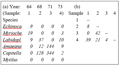
Table 2.1a shows the data matrix of counts and Table 2.1b the resulting lower triangular matrix of Bray-Curtis similarity coefficients. For example, using the first form of equation (2.1), the similarity between samples 1 and 4 (years 1964 and 1973) is:

$$S_{14} = 100 \left[ 1 - \frac{9+16+1+9+2+0}{9+22+19+9+2+0} \right] = 39.3 $$

The second form of equation (2.1) can be seen to give the same result:

$$S_{14} = 100 \left[\frac{2[0+3+9+0+0+0]}{9+22+19+9+2+0} \right] = 39.3 $$

Computation is therefore simple and it is easy to verify that the coefficient possesses the following desirable properties.

a) S = 0 if the two samples have no species in common, since min ($y_{ij}$, $y_{ik}$) = 0 for all i (e.g. samples 1 and 3 of Table 2.1a). Of course, S = 100 if two samples are identical, since |$y_{ij} - y_{ik}$| = 0 for all i.

b) A scale change in the measurements does not change S. For example, biomass could be expressed in g rather than mg or abundance changed from numbers per cm$^2$ of sediment surface to numbers per m$^2$; all y values are simply multiplied by the same constant and this cancels in the numerator and denominator terms of equation (2.1).

c) ‘Joint absences’ also have no effect on S. In Table 2.1a the last species is absent in all samples; omitting this species clearly makes no difference to the two summations in equation (2.1). That similarity should depend on species which are present in one or other (or both) samples, and not on species which are absent from both, is usually a desirable property. As Field, Clarke & Warwick (1982) put it: "taking account of joint absences has the effect of saying that estuarine and abyssal samples are similar because both lack outer-shelf species”. Note that a lack of dependence on joint absences is by no means a property shared by all similarity coefficients.

Transformation of raw data

In one or two ways, the similarities of Table 2.1b are not a good reflection of the overall match between the samples, taking all species into account. To start with, the similarities all appear too low; samples 2 and 3 would seem to deserve a similarity rating higher than 50%. As will be seen later, this is not an important consideration since most of the multivariate methods in this manual depend only on the relative order (ranking) of the similarities in the triangular matrix, rather than their absolute values. More importantly, the similarities of Table 2.1b are unduly dominated by counts for the two most abundant species (4 and 5), as can be seen from studying the form of equation (2.1): terms involving species 4 and 5 will dominate the sums in both numerator and denominator. Yet the larger abundances in the original data matrix will often be extremely variable in replicate samples (the issue of variance structures in community data is returned to in Chapter 9) and it is usually undesirable to base an assessment of similarity of two communities only on the counts for a handful of very abundant species.

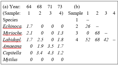
The answer is to transform the original y values (the counts, biomass, % cover or whatever) before computing the Bray-Curtis similarities. Two useful transformations are the root transform, $\sqrt{}$y, and the double root (or 4th root) transform, $\sqrt{}\sqrt{}$y. There is more on the effects of transformation later, in Chapter 9; for now it is only necessary to note that the root transform, $\sqrt{}$y, has the effect of down-weighting the importance of the highly abundant species, so that similarities depend not only on their values but also those of less common (‘mid-range’) species. The 4th root transform, $\sqrt{}\sqrt{}$y, takes this process further, with a more severe down-weighting of the abundant species, allowing not only the mid-range but also the rarer species to exert some influence on the calculation of similarity. An alternative severe transformation, with very similar effect to the 4th root, is the log transform, log(1+y).

The result of the 4th root transform for the previous example is shown in Table 2.2a, and the Bray-Curtis similarities computed from these transformed abundances, using equation (2.1), are given in Table 2.2b.^‡ There is a general increase in similarity levels but, of more importance, the rank order of similarities is no longer the same as in Table 2.1b (e.g. $S _ {24} > S _ {14}$ and $S _ {34} > S _ {12}$ now), showing that transformations can have a significant effect on the final multivariate display.

Table 2.2. Loch Linnhe macrofauna {L} subset. (a) $\sqrt{}\sqrt{}$-transformed abundance for the four years and six species of Table 2.1. (b) Resulting Bray-Curtis similarity matrix.

In fact, choice of transformation can be more important than level of taxonomic identification (see Chapter 16) especially when abundances are extreme, such as for highly-clumped or schooling species, when dispersion weighting, in place of (or prior to) transformation can be an effective strategy, see Chapter 9.

Canberra coefficient

An alternative which also reduces variability and may sometimes eliminate the need for transformation^§ is to select a similarity measure that automatically balances the weighting given to each species when computed on original counts. One such possibility, the Stephenson, Williams & Cook (1972) form of the so-called Canberra coefficient of Lance & Williams (1967) , defines the similarity between samples j and k as:

$$S_{jk} = 100 \left[ 1 - \frac{1}{p} \sum_{i=1}^{p} \frac{| y_{ij} - y_{ik} | }{( y_{ij} + y_{ik} ) } \right] \tag{2.2}$$

This is another member of the ‘Bray-Curtis family’, bearing a strong likeness to (2.1), but the absolute differences in counts for each species are separately scaled, i.e. the denominator scaling term is inside not outside the summation over species. For example, from Table 2.1a, the Canberra similarity between samples 1 and 4 is:

$$S_{14} = 100 \left[ 1 -\frac{1}{5} \left( \frac{9}{9} + \frac{16}{22} + \frac{1}{19} +\frac{9}{9} +\frac{2}{2} \right) \right] = 24.4 $$

Note that joint absences have no effect here because they are deliberately excluded (since 0/0 is undefined) and p is reset to be the number of species that are present in at least one of the two samples under consideration, an important step for a number of biological measures.

The separate scaling constrains each species to make equal contribution (potentially) to the similarity between two samples. However abundant a species is, its contribution to S can never be more than 100/p, and a rare species with a single individual in each of the two samples contributes the same as a common species with 1000 individuals in each. Whilst there may be circumstances in which this is desirable, more often it leads to overdomination of the pattern by a large number of rare species, of no real significance. (Often the sampling strategy is incapable of adequately quantifying the rarer species, so that they are distributed arbitrarily, to some degree, across the samples.)

Correlation coefficient

A common statistical means of assessing the relationship between two columns of data (samples j and k here) is the standard product moment, or Pearson, correlation coefficient:

$$r_{jk} = \frac{\sum_i ( y_{ij} - \overline{y} _ {\bullet j})( y_{ik} - \overline{y} _ {\bullet k}) } {\sqrt{ \sum_i ( y_{ij} - \overline{y} _ {\bullet j})^2 \sum_i ( y_{ik} - \overline{y} _ {\bullet k})^2}} \tag{2.3}$$

where $ \overline{y} _ {\bullet j}$ is defined as the mean value over all species for the jth sample. In this form it is not a similarity coefficient, since it takes values in the range (–1, 1), not (0, 100), with positive correlation (r near +1) if high counts in one sample match high counts in the other, and negative correlation (r < 0) if high counts match absences. There are a number of ways of converting r to a similarity coefficient, the most obvious for community data being S = 50(1+r).

Whilst correlation is sometimes used as a similarity coefficient, it is not particularly suitable for much biological community data, with its plethora of zero values. For example, it violates the criterion that S should not depend on joint absences; here two columns are more highly positively correlated (and give S nearer 100) if species are added which have zero counts for both samples. If correlation is to be used a measure of similarity, it makes good sense to transform the data initially, exactly as for the Bray-Curtis computation, so that large counts or biomass do not totally dominate the coefficient.

General suitability of Bray-Curtis

The ‘Bray-Curtis family’ is defined by Clarke, Somerfield & Chapman (2006) as any similarity which satisfies all of the following desirable, ecologically-oriented guidelines^¶

a) takes the value 100 when two samples are identical (applies to most coefficients);

b) takes the value 0 when two samples have no species in common (this is a much tougher condition and most coefficients do not obey it);

c) a change of measurement unit does not affect its value (most coefficients obey this one);

d) value is unchanged by inclusion or exclusion of a species which is jointly absent from the two samples (another difficult condition to satisfy, and many coefficients do not obey this one);

e) inclusion (or exclusion) of a third sample, C, in the data array makes no difference to the similarity between samples A and B (several coefficients do not obey this, because they depend on some form of standardisation carried out for each species, by the species total or maximum across all samples);

f) has the flexibility to register differences in total abundance for two samples as a less-than-perfect similarity when the relative abundances for all species are identical (some coefficients standardise automatically by sample totals, so cannot reflect this component of similarity/difference).

In addition, Faith, Minchin & Belbin (1987) use a simulation study to look at the robustness of various similarity coefficients in reconstructing a (non-linear) ecological response gradient. They find that Bray-Curtis and a very closely-related modification (also in the Bray-Curtis family), the Kulczynski coefficient

$$S_{jk} = 100 \frac{\sum _ {i=1} ^ p \min ( y_{ij}, y_{ik}) } {2 / \left[ \left( \sum _ {i=1} ^ p y_{ij} \right) ^ {-1} + \left( \sum _ {i=1} ^ p y_{ij} \right) ^ {-1} \right] } \tag{2.4}$$

Kulczynski (1928) , perform most satisfactorily^†.

Coefficients other than Bray-Curtis, which satisfy all of the above conditions, tend either to have counterbalancing drawbacks, such as the Canberra measure’s forced equal weighting of rare and common species, or to be so closely related to Bray-Curtis as to make little practical difference to most analyses, such as the Kulczynski coefficient, which clearly reverts to Bray-Curtis exactly for standardised samples (when sample totals are all 100).

---

^‡ After a range of Pre-treatment options (including transformation) Bray-Curtis is the default coefficient in the PRIMER Resemblance routine, on data defined as type Abundance (or Biomass), but PRIMER also offers nearly 50 other resemblance measures.

^§ This removes all differences across species in terms of absolute mean abundance but does not address erratic differences within species resulting from schooled or clumped arrivals over the samples. The converse is true of dispersion weighting.

^¶ They are not, of course, universally accepted as desirable! In non-ecological contexts there may be no concept of zero as a ‘special’ number, which must be preserved under transformation because it indicates absence of a species (and ecological work is often concerned as much with the balance of species that are present or absent, as it is with the numbers of individuals found). Even in ecological contexts, some authors prefer not to use a coefficient which has a finite limit (100% = perfect dissimilarity), in part because of technical difficulties this may cause for parametric or semi-parametric modelling when there are many samples with no species in common. These technical issues do not arise for the flexible rank-based methods advocated here (such as non-metric multi-dimensional scaling ordination).

^† This is simply the second form of the Bray-Curtis definition in (2.1), with the denominator terms of the arithmetic mean of the two sample totals across species, $(f+g)/2$, being replaced with a harmonic mean, $2/ ( f^{-1} + g^{-1} )$. In the current authors’ experience, this behaves slightly less well than Bray-Curtis because of the way a harmonic mean is strongly dragged towards the smallest of the totals f and g. Clarke, Somerfield & Chapman (2006) define an intermediate option (also therefore in the Bray-Curtis family) which has a geometric mean divisor $(fg) ^ {0.5}$. This is termed quantitative Ochiai because it reduces to a well-known measure ( Ochiai (1957) ) when the data are only of presences or absences. The serious point here is that it is sufficiently easy to produce new, sensible similarity coefficients that some means of summarising their ‘similarity’ to each other, in terms of their effects on a multivariate analysis, is essential. This is deferred until the 2nd stage plots of Chapter 16.

2.3 Presence/absence data

As discussed at the beginning of this chapter, quantitative uncertainty may make it desirable to reduce the data simply to presence or absence of each species in each sample, or this may be the only feasible or cost-effective option for data collection in the first place. Alternatively, reduction to presence/absence may be thought of as the ultimate in severe transformation of counts; the data matrix (e.g. in Table 2.1a) is replaced by 1 (presence) or 0 (absence) and Bray-Curtis similarity (say) computed. This will have the effect of giving potentially equal weight to all species, whether rare or abundant (and will thus have somewhat similar effect to the Canberra coefficient, a suggestion confirmed by the comparative analysis in Chapter 16).

Many similarity coefficients have been proposed based on (0, 1) data arrays; see for example, Sneath & Sokal (1973) or Legendre & Legendre (2012) . When computing similarity between samples j and k, the two columns of data can be reduced to the following four summary statistics without any loss of relevant information:

a = the number of species which are present in both samples;

b = the number of species present in sample j but absent from sample k;

c = the number of species present in sample k but absent from sample j;

d = the number of species absent from both samples.

For example, when comparing samples 1 and 4 from Table 2.1a, these frequencies are:

		Sample 4:	1	0
Sample 1:	1		a = 2	b = 1
	0		c = 2	d = 1

In fact, because of the symmetry, coefficients must be a symmetric function of b and c, otherwise $S _ {14}$ will not equal $S _ {41}$. Also, similarity measures not affected by joint absences will not contain d. The following are some of the more commonly advocated coefficients.

The simple matching similarity between samples j and k is defined as:

$$ S _ {jk} = 100 \left[ (a + d) / (a + b + c + d) \right] \tag{2.5} $$

so called because it represents the probability ($\times 100$) of a single species picked at random (from the full species list) being present in both samples or absent in both samples. Note that S is a function of d here, and thus depends on joint absences.

If the simple matching coefficient is adjusted, by first removing all species which are jointly absent from samples j and k, one obtains the Jaccard coefficient:

$$ S _ {jk} = 100 \left[ a / (a + b + c ) \right] \tag{2.6} $$

i.e. S is the probability ($\times 100$) that a single species picked at random (from the reduced species list) will be present in both samples.

A popular coefficient found under several names, commonly Sørensen or Dice, is

$$ S _ {jk} = 100 \left[ 2a / (2a + b + c ) \right] \tag{2.7} $$

Note that this is identical to the Bray-Curtis coefficient when the latter is calculated on (0, 1) presence/absence data, as can be seen most clearly from the second form of equation (2.1).^¶ For example, reducing Table 2.1a to (0, 1) data, and comparing samples 1 and 4 as previously, equation (2.1) gives:

$$S_{14} = 100 \left[ \frac{2(0+1+1+0+0+0)}{1+2+2+1+1+0} \right] = 57.1 $$

This is clearly the same construction as substituting a = 2, b = 1, c = 2 into equation (2.7).

Several other coefficients have been proposed; Legendre & Legendre (2012) list at least 15, but only one further measure is given here. In the light of the earlier discussion on coefficients satisfying desirable, biologically-motivated criteria, note that there is a presence/absence form of the Kulczynski coefficient (2.4), a close relative of Bray-Curtis/Sørensen, namely:

$$S _ {jk} = 50 \left( \frac{a}{a+b} + \frac{a}{a+c} \right) \tag{2.8} $$

Recommendations

1. In most ecological studies, some intuitive axioms for desirable behaviour of a similarity coefficient lead to the use of the Bray-Curtis coefficient (or a closely-related measure such as Kulczynski).

2. Similarities calculated on original abundance (or biomass) values can often be over-dominated by a small number of highly abundant (or large-bodied) species, so that they fail to reflect similarity of overall community composition.

3. Some coefficients (such as Canberra and that of Gower (1971) , see later), which separately scale the contribution of each species to adjust for this, have a tendency to over-compensate, i.e. rare species, which may be arbitrarily distributed across the samples, are given equal weight to abundant ones. The same criticism applies to reduction of the data matrix to simple presence/absence of each species. In addition, the latter loses potentially valuable information about the approximate numbers of a species (0: absent, 1: singleton, 2: present only as a handful of individuals, 3: in modest numbers, 4: in sizeable numbers; 5: abundant; 6: highly abundant. This apparently crude scale can often be just as effective as analysing the precise counts in a multivariate analysis, which typically extracts a little information from a lot of species).

4. A balanced compromise is often to apply the Bray-Curtis similarity to counts (or biomass, area cover etc) which have been moderately, $\sqrt{}$y, or fairly severely transformed, log(1+y) or $\sqrt{} \sqrt{}$y (i.e. $y ^ {0.25}$). Most species then tend to contribute something to the definition of similarity, whilst the retention of some information on species numbers ensures that the more abundant species are given greater weight than the rare ones. A good way of assessing where this balance lies – how much of the matrix is being used for any specific transformation – is to view shade plots of the data matrix, as seen in Figs. 7.7 to 7.10 and 9.5 and 9.6.

5. Pre-treating the data, prior to transformation, by standardisation of samples is sometimes desirable, depending on the context. This divides each count by the total abundance of all species in that sample and multiplies up by 100 to give a percent composition (or perhaps standardises by the maximum abundance). Worries that this somehow makes the species variables non-independent, since they must now add to 100, are misplaced: species variables are always non-independent – that is the point of multivariate analysis! Without sample standardisation, the Bray-Curtis coefficient will reflect both compositional differences among samples and (to a weak extent after transformation) changing total abundance at the different sites/times/treatments.^§

---

^¶ Thus the Sorensen coefficient can be obtained in two ways in the PRIMER Resemblance routine, either by taking S8 Sorensen in the P/A list or by transforming the data to presence/absence and selecting Bray-Curtis similarity.

^§ The latter is usually thought necessary, by marine benthic ecologists at least: if everything becomes half as abundant they want to know about it! However, much depends on the sampling device and the patchiness of biota; plankton ecologists usually do standardise, as will kick-samplers in freshwater, where there is much less control of ‘sample volume’. Standardisation removes any contribution from totals but it does not remove the subsequent need to transform, in order to achieve a better balance of the abundant and rarer species.

2.4 Species similarities

Starting with the original data matrix of abundances (or biomass, area cover etc), the similarity between any pair of species can be defined in an analogous way to that for samples, but this time involving comparison of the ith and lth row (species) across all j = 1, ..., n columns (samples).

Bray-Curtis coefficient

The Bray-Curtis similarity between species i and l is:

$$S _ {il} ^ \prime = 100 \left[ 1 - \frac{\sum_{j=1}^{n} | y_{ij} - y_{lj} | }{\sum_{j=1}^{n} ( y_{ij} + y_{lj} ) } \right] \tag{2.9}$$

The extreme values are (0, 100) as previously:

$S ^ \prime = 0 $ if two species have no samples in common (i.e. are never found at the same sites)

$S ^ \prime= 100$ if the y values for two species are the same at all sites

However, different initial treatment of the data is required, in two respects.

1. Similarities between rare species have little meaning; very often such species have single occurrences, distributed more or less arbitrarily across the sites, so that S′ is usually zero (or occasionally 100). If these values are left in the similarity matrix they will tend to confuse and disrupt the patterns in any subsequent multivariate analysis; the rarer species should thus be omitted from the data matrix before computing species similarities.

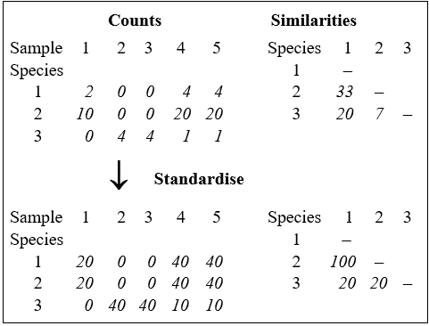
2. A different form of standardisation (species standardisation) of the data matrix is relevant and, in contrast to the samples analysis, it usually makes sense to carry this out routinely, usually in place of a transformation^¶. Two species could have quite different mean levels of abundance yet be perfectly similar in the sense that their counts are in strict ratio to each other across the samples. One species might be of much larger body size, and thus tend to have smaller counts, for example; or there might be a direct host-parasite relationship between the two species. It is therefore appropriate to standardise the original data by dividing each entry by its species total over samples, and multiplying by 100:

$$y _ {ij} ^ \prime = 100 y _ {ij} / \sum_{k=1}^{n} y_{ik} \tag{2.10}$$

before computing the similarities ($S ^ \prime$). The effect of this can be seen from the artificial example in the following table, for three species and five samples. For the original matrix, the Bray-Curtis similarity between species 1 and 2, for example, is only $S ^ \prime = 33$% but the two species are found in strict proportion to each other across the samples so that, after row standardisation, they have a more realistic similarity of $S ^ \prime = 100$%.

Correlation coefficient

The standard product moment correlation coefficient defined in equation (2.3), and subsequently modified to a similarity, is perhaps more appropriate for defining species similarities than it was for samples, in that it automatically incorporates a type of row standardisation. In fact, this is a full normalisation (subtracting the row mean from each count and dividing by the row standard deviation) and it is less appropriate than the simple row standardisation above. One of the effects of normalisation here is to replace zeros in the matrix with largish negative values which differ from species to species – the presence/absence structure is entirely lost. The previous argument about the effect of joint absences is equally appropriate to species similarities: an inter-tidal species is no more similar to a deep-sea species because neither is found in shelf samples. A correlation coefficient will again be a function of joint absences; the Bray-Curtis coefficient will not.

Recommendation

For species similarities, a coefficient such as Bray-Curtis calculated on row-standardised and untransformed data seems most appropriate. The rarer species (often at least half of the species set) should first be removed from the matrix, to have any chance of an interpretable multivariate clustering or other analysis. There are several ways of doing this, all of them arbitrary to some degree. Field, Clarke & Warwick (1982) suggest removal of all species that never constitute more than q% of the total abundance (/biomass/cover) of any sample, where q is chosen to retain around 50 or 60 species (typically q = 1 to 3%, for benthic macrofauna samples). This is preferable to simply retaining the 50 or 60 species with the highest total abundance over all samples, since the latter strategy may result in omitting several species which are key constituents of a site which is characterised by a low total number of individuals.^§ It is important to note, however, that this inevitably arbitrary process of omitting species is not necessary for the more usual between-sample similarity calculations. There the computation of the Bray-Curtis coefficient downweights the contributions of the less common species in an entirely natural and continuous fashion (the rarer the species the less it contributes, on average), and all species should be retained in those calculations.

---

^¶ Species standardisation will remove the typically large overall abundance differences between species (which is one reason we needed transformation for a samples analysis, which dilutes this effect without removing it altogether) but it does not address the issue of large outliers for single species across samples. Transformations might help here but, in that case, they should be done before the species standardisation.

^§ The PRIMER Resemblance routine will compute Bray-Curtis species similarities, though you need to have previously species- standardised the matrix (by totals) in the Pre-treatment routine. An alternative is to directly calculate Whittaker’s Index of Association on the species, see equation (7.1), since this is the same calculation except that it includes the standardisation step as part of the coefficient definition. (As Chapter 7 shows, if you are planning on using the SIMPROF test on species, described there, species standardisation is still needed). Prior to this, the Select Variables option allows reduction of the number of species, by retaining those that contribute q% or more to at least one of the samples, or by specifying the number n of ‘most important’ species to retain. The latter uses the same q% criterion but gradually increases q until only n species are left.

2.5 Dissimilarity coefficients

The converse concept to similarity is that of dissimilarity, the degree to which two samples are unlike each other. As previously stated, similarities (S) can be turned into dissimilarities ($\delta$), simply by:

$$ \delta = 100 -S \tag{2.11} $$

which of course has limits $\delta = 0$ (no dissimilarity) and $\delta = 100$ (total dissimilarity). $\delta$ is a more natural starting point than S when constructing ordinations, in which dissimilarities between pairs of samples are turned into distances (d) between sample locations on a ‘map’ – the highest dissimilarity implying, naturally, that the samples should be placed furthest apart.

Bray-Curtis dissimilarity is thus defined by (2.1) as:

$$\delta_{jk} = 100 \frac{\sum_{i=1}^{p} | y_{ij} - y_{ik} | }{\sum_{i=1}^{p} ( y_{ij} + y_{ik} ) } \tag{2.12}$$

However, rather than conversion from similarities, other important measures arise in the first place as dissimilarities, or more often distances, the key difference between the latter being that distances are not limited to a finite range but defined over (0, $\infty$). They may be calculated explicitly or have an implicit role as the distance measure underlying a specific ordination method, e.g. as Euclidean distance is for PCA (Principal Components Analysis, Chapter 4) or chi-squared distance for CA (Correspondence Analysis).

Euclidean distance

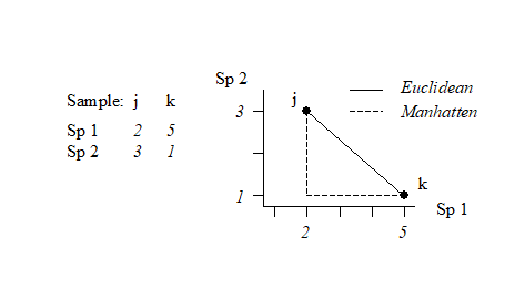
The natural distance between any two points in space is referred to as Euclidean distance (from classical or Euclidean geometry). In the context of a species abundance matrix, the Euclidean distance between samples j and k is defined algebraically as:

$$d_{jk} = \sqrt{\sum_{i=1}^{p} ( y_{ij} - y_{ik} )^2 } \tag{2.13}$$

This can best be understood, geometrically, by taking the special case where there are only two species so that samples can be represented by points in 2-dimensional space, namely their position on the two axes of Species 1 and Species 2 counts. This is illustrated below for a simple two samples by two species abundance matrix. The co-ordinate points (2, 3) and (5, 1) on the (Sp. 1, Sp. 2) axes are the two samples j and k. The direct distance $d_{jk}$ between them of $\sqrt{(2–5)^2 + (3–1)^2}$ (from Pythagoras) clearly corresponds to equation (2.13).

It is easy to envisage the extension of this to a matrix with three species; the two points are now simply located on 3-dimensional species axes and their straight line distance apart is a natural geometric concept. Algebraically, it is the root of the sums of squared distances apart along the three axes, equation (2.13) –Pythogoras applies in any number of dimensions! Extension to four and higher numbers of species (dimensions) is harder to envisage geometrically, in our 3-dimensional world, but the concept remains unchanged and the algebra is no more difficult to understand in higher dimensions than three: additional squared distances apart on each new species axis are added to the summation under the square root in equation (2.13). In fact, this concept of representing a species-by-samples matrix as points in high-dimensional species space is a very fundamental and important one and will be met again in Chapter 4, where it is crucial to an understanding of Principal Components Analysis.

Manhattan distance

Euclidean distance is not the only way of defining distance apart of two samples in species space; an alternative is to sum the distances along each species axis:

$$d_{jk} = \sum_{i=1}^{p} | y_{ij} - y_{ik} | \tag{2.14}$$

This is often referred to as Manhattan (or city-block) distance because in two dimensions it corresponds to the distance you would have to travel to get between any two locations in a city whose streets are laid out in a rectangular grid. It is illustrated in the simple figure above by the dashed lines. Manhattan distance is of interest here because of its obvious close affinity to Bray-Curtis dissimilarity, equation (2.12). In fact, when a data matrix has initially been sample standardised (but not transformed), Bray-Curtis dissimilarity is just (half) the Manhattan distance, since the summation in the bottom line of (2.12) then always takes the value 200.

In passing, it is worth noting a point of terminology, though not of any great practical consequence for us. Euclidean and Manhattan measures, equations (2.13) and (2.14), are known as metrics because they obey the triangle inequality, i.e. for any three samples j, k, r:

$$ d _ {jk} + d _ {kr} \ge d_{jr} \tag{2.15} $$

Bray-Curtis dissimilarity does not, in general, satisfy the triangle inequality, so should not be called a metric. However, many other useful coefficients are also not metric distances. For example, the square of Euclidean distance (i.e. equation (2.13) without the $\sqrt{}$ sign) is another natural definition of ‘distance’ which is not a metric, yet the values from this would have the same rank order as those from Euclidean distance and thus give rise, for example, to identical MDS ordinations (Chapter 5). It follows that whether a dissimilarity coefficient is, or is not, a metric is likely to be of no practical significance for the non-parametric (rank-based) strategy that this manual generally advocates.^¶

---

^¶ Though it is of slightly more consequence for the Principal Co-ordinates Analysis ordination, PCO, and the semi-parametric modelling framework of the add-on PERMANOVA+ routines to PRIMER, see Anderson, Gorley & Clarke (2008) , page 110.

2.6 More on resemblance measures

On the grounds that it is better to walk before you try running, discussion of comparisons between specific similarity, dissimilarity and distance coefficients, that the PRIMER software refers to generally by the term resemblance measures, is left until after presentation of a useful suite of multivariate analyses that can be generated from a given set of sample resemblances, and then how such sets of resemblances themselves can be compared (second-stage analysis, Chapter 16). One topic can realistically be addressed here, though.

Missing data and resemblance calculation

Missing data in this context does not mean missing whole samples (e.g. the intention was to collect five replicates but at one location only four were taken). The latter is better described as unbalanced sampling design and is handled automatically, and without difficulty, by most of the methods in this manual (an exception is when trying to link the biotic assemblage at a site to a set of measured environmental variables, e.g. in the BEST routine of Chapter 11, where a full match is required). Missing data here means missing values for only some of the combinations of variables (species) and samples. As such, it is more likely to occur for environmental-type variables or – to take an entirely different type of data – questionnaire returns. There, the variables are the different questions and the samples the people completing the questionnaire, and missing answers to questions are commonplace.

Of course, one solution is to omit some combination of variables and samples such that a complete matrix results, but this might throw away a great deal of the data. Separately for each sample pair whose resemblance is being calculated, one could eliminate any variables with a missing value in either sample (this is known as pairwise elimination of missing values). But this can be biased for some coefficients, e.g. the Euclidean distance (2.13) sums the (squared) contributions from each variable; if several variables have to be omitted for one distance calculation, but none are left out for a second distance, then the latter will be an (artefactually) larger distance, inevitably. The same will be true of, for example, Manhattan distance but not of some other measures, such as Bray-Curtis or average Euclidean (which divides the Euclidean distance by p’, the fluctuating number of terms being summed over) – in fact for anything which behaves more like an average of contributions rather than a sum. An approximate correction for this crude bias can be made for all coefficients, where necessary.^†

Variable weighting in resemblance calculation

We have already mentioned the effects of transformation on the outcome of a resemblance calculation and Chapter 9 discusses this in more detail, ending with a description of another important pre-treatment method, as an alternative to (or precursor of) transforming abundances, viz. the differential weighting of species by dispersion weighting. This down-weights species whose counts are shown to be unreliable in replicates of the same site/time/condition, i.e. they have a high variance-to-mean ratio (dispersion index) over such replicates. The solution, in a quite general way, is to downweight each species contribution by the dispersion index, averaged over replicates. In a rather similar idea, variables can be subjected to variability weighting, in which downweighting is not by the index of dispersion (suitable for species count data) but by the average standard deviation^¶ over replicates. This is relevant to variables like indices (of diversity, health etc, see Hallett, Valesini & Clarke (2012) ) and results in more weight being given to indices which are more reliable in repeated measurement. A final possibility in PRIMER is just to weight variables according to some pre-defined scale, e.g. in studies of coral communities by amateur divers, Mumby, Clarke & Harborne (1996) give an example in which some species are often misidentified, with known rates calibrated against professional assessments; these species are thus downweighted in the resemblance calculation.

Recommendations

Thus, depending on the type of data, there are a variety of means to generate a resemblance matrix (similarity, dissimilarity or distance) to input to the next stage of a multivariate analysis, which might be either a clustering or ordination of samples, Fig. 2.1. For comparative purposes it may sometimes be of interest to use Euclidean distance in the species space as input to a cluster analysis** (an example is given later in Fig. 5.5) but, in general, the recommendation remains unchanged: Bray-Curtis similarity/dissimilarity, computed after suitable transformation, will often be a satisfactory coefficient for biological data of community structure. That is, use Bray-Curtis, or one of the closely related coefficients satisfying the criteria given on page 2.2 (the ‘Bray-Curtis family’ of Clarke, Somerfield & Chapman (2006) ) for data in which it is important to capture the structure of presences and absences in the samples in addition to the quantitative counts (or density/biomass/area cover etc) of the species which are present. Background physical or chemical data is a different matter since it is usually of a rather different type, and Chapter 11 shows the usefulness of the idea of linking to environmental variable space, assessed by Euclidean distance on normalised data. The first step though is to calculate resemblances for the biotic data on its own, followed by a cluster analysis or ordination (Fig. 2.1).

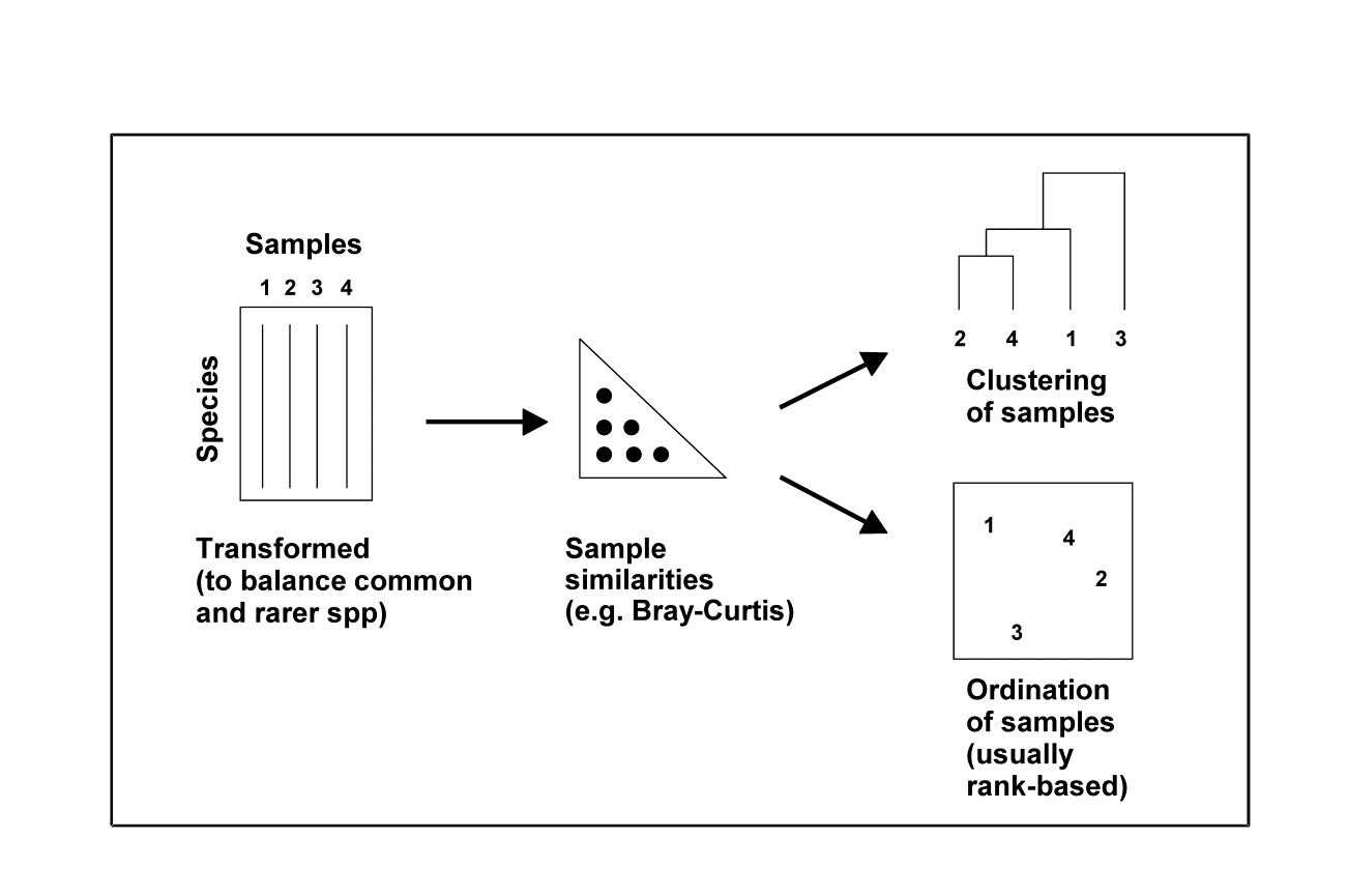
Fig. 2.1. Stages in a multivariate analysis based on (dis)similarity coefficients.

---

^† Earlier PRIMER versions did not offer this, but v7 makes this bias correction for all coefficients that need it, e.g. for standard Euclidean distance, the pairwise-eliminated distance is multiplied by $\sqrt{p/p^\prime}$, where $p$ is the (fixed) number of variables in the matrix and $p^\prime$ the (differing) number of retained pairs for each specific distance. Manhattan uses factor $(p/p^\prime)$ but the Bray-Curtis family does not need it.

^¶ The PRIMER Pre-treatment menu, under Variability Weighting, offers the choice between dividing each species through by its average replicate range, inter-quartile (IQ) range, standard deviation (SD) or pooled SD (as would be calculated in ANOVA from a common variance estimate, then square rooted). Note that this weighting uses only variability within factor levels not across the whole sample set, as in normalisation (dividing by overall SD). Clearly, variability weighting is only applicable when there are replicate samples, and these must be genuinely independent of each other, properly capturing the variability at each factor level, for the technique to be meaningful.