Chapter 3: Clustering methods
- 3.1 Cluster analysis
- 3.2 Hierarchical agglomerative clustering
- 3.3 Example: Bristol Channel zooplankton
- 3.4 Recommendations
- 3.5 Similarity profiles (SIMPROF)
- 3.6 Binary divisive clustering
- 3.7 k-R clustering (non-hierarchical)
3.1 Cluster analysis
The previous chapter has shown how to replace the original data matrix with pairwise similarities, chosen to reflect the particular aspect of community similarity of interest for that study (similarity in counts of abundant species, similarity in location of rare species etc). Typically, the number of pairwise similarities is large, n(n–1)/2 for n samples, and it is difficult visually to detect a pattern in the triangular similarity matrix. Table 3.1 illustrates this for just part (roughly a quarter) of the similarity matrix for the Frierfjord macrofauna data {F}. Close examination shows that the replicates within site A generally have higher within-site similarities than do pairs of replicates within sites B and C, or between-site samples, but the pattern is far from clear. What is needed is a graphical display linking samples that have mutually high levels of similarity.
Table 3.1. Frierfjord macrofauna counts {F}. Bray-Curtis similarities, on $\sqrt{}\sqrt{}$-transformed counts, for every pair of replicate samples from sites A, B, C only (four replicate samples per site).
| A1 | A2 | A3 | A4 | B1 | B2 | B3 | B4 | C1 | C2 | C3 | C4 | |
|---|---|---|---|---|---|---|---|---|---|---|---|---|
| A1 | – | |||||||||||
| A2 | 61 | – | ||||||||||
| A3 | 69 | 60 | – | |||||||||
| A4 | 65 | 61 | 66 | – | ||||||||
| B1 | 37 | 28 | 37 | 35 | – | |||||||
| B2 | 42 | 34 | 31 | 32 | 55 | – | ||||||
| B3 | 45 | 39 | 39 | 44 | 66 | 66 | – | |||||
| B4 | 37 | 29 | 29 | 37 | 59 | 63 | 60 | – | ||||
| C1 | 35 | 31 | 27 | 25 | 28 | 56 | 40 | 34 | – | |||
| C2 | 40 | 34 | 26 | 29 | 48 | 69 | 62 | 56 | 56 | – | ||
| C3 | 40 | 31 | 37 | 39 | 59 | 61 | 67 | 53 | 40 | 66 | – | |
| C4 | 36 | 28 | 34 | 37 | 65 | 55 | 69 | 55 | 38 | 64 | 74 | – |
Cluster analysis (or classification, see footnote on terminology on page 1.2) aims to find natural groupings of samples such that samples within a group are more similar to each other, generally, than samples in different groups. Cluster analysis is used in the present context in the following ways.
a) Different sites (or different times at the same site) can be seen to have differing community compositions by noting that replicate samples within a site form a cluster that is distinct from replicates within other sites. This can be an important hurdle to overcome in any analysis; if replicates for a site are clustered more or less randomly with replicates from every other site then further interpretation is likely to be dangerous. (A more formal statistical test for distinguishing sites is the subject of Chapter 6).
b) When it is established that sites can be distinguished from one another (or, when replicates are not taken, it is assumed that a single sample is representative of that site or time), sites or times can be partitioned into groups with similar community structure.
c) Cluster analysis of the species similarity matrix can be used to define species assemblages, i.e. groups of species that tend to co-occur in a parallel manner across sites.
Range of methods
Literally hundreds of clustering methods exist, some of them operating on similarity/dissimilarity matrices whilst others are based on the original data. Everitt (1980) and Cormack (1971) give excellent and readable reviews. Clifford & Stephenson (1975) is another well-established text from an ecological viewpoint.
Five classes of clustering methods can be distinguished, following the categories of Cormack (1971) .
-
Hierarchical methods. Samples are grouped and the groups themselves form clusters at lower levels of similarity.
-
Optimising techniques. A single set of mutually exclusive groups (usually a pre-specified number) is formed by optimising some clustering criterion, for example minimising a within-cluster distance measure in the species space.
-
Mode-seeking methods. These are based on considerations of density of samples in the neighbourhood of other samples, again in the species space.
-
Clumping techniques. The term ‘clumping’ is reserved for methods in which samples can be placed in more than one cluster.
-
Miscellaneous techniques.
Cormack (1971) also warned against the indiscriminate use of cluster analysis: “availability of … classification techniques has led to the waste of more valuable scientific time than any other ‘statistical’ innovation”. The ever larger number of techniques and their increasing accessibility on modern computer systems makes this warning no less pertinent today. The policy adopted here is to concentrate on a single technique that has been found to be of widespread utility in ecological studies, whilst emphasising the potential arbitrariness in all classification methods and stressing the need to perform a cluster analysis in conjunction with a range of other techniques (e.g. ordination, statistical testing) to obtain balanced and reliable conclusions.
3.2 Hierarchical agglomerative clustering
The most commonly used clustering techniques are the hierarchical agglomerative methods. These usually take a similarity matrix as their starting point and successively fuse the samples into groups and the groups into larger clusters, starting with the highest mutual similarities then lowering the similarity level at which groups are formed, ending when all samples are in a single cluster. Hierarchical divisive methods perform the opposite sequence, starting with a single cluster and splitting it to form successively smaller groups.
The result of a hierarchical clustering is represented by a tree diagram or dendrogram, with the x axis representing the full set of samples and the y axis defining a similarity level at which two samples or groups are considered to have fused. There is no firm convention for which way up the dendrogram should be portrayed (increasing or decreasing y axis values) or even whether the tree can be placed on its side; all three possibilities can be found in this manual.
Fig. 3.1 shows a dendrogram for the similarity matrix from the Frierfjord macrofauna, a subset of which is in Table 3.1. It can be seen that all four replicates from sites A, D, E and G fuse with each other to form distinct site groups before they amalgamate with samples from any other site; that, conversely, site B and C replicates are not distinguished, and that A, E and G do not link to B, C and D until quite low levels of between-group similarities are reached.
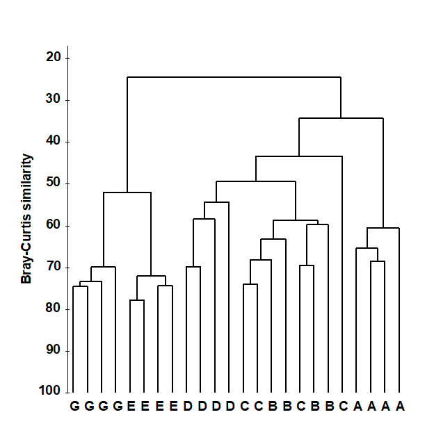
Fig. 3.1. Frierfjord macrofauna counts {F}. Dendrogram for hierarchical clustering (using group-average linking) of four replicate samples from each of sites A-E, G, based on the Bray- Curtis similarity matrix shown (in part) in Table 3.1.
The mechanism by which Fig. 3.1 is extracted from the similarity matrix, including the various options for defining what is meant by the similarity of two groups of samples, is best described for a simpler example.
Construction of dendrogram
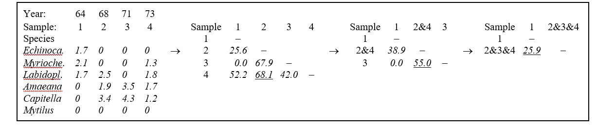
Table 3.2 shows the steps in the successive fusing of samples, for the subset of Loch Linnhe macrofaunal abundances used as an example in the previous chapter. The data matrix has been $\sqrt{}\sqrt{}$-transformed, and the first triangular array is the Bray-Curtis similarity of Table 2.2.
Samples 2 and 4 are seen to have the highest similarity (underlined) so they are combined, at similarity level 68.1%. (Above this level there are considered to be four clusters, simply the four separate samples.) A new similarity matrix is then computed, now containing three clusters: 1, 2&4 and 3. The similarity between cluster 1 and cluster 3 is unchanged at 0.0 of course but what is an appropriate definition of similarity S(1, 2&4) between clusters 1 and 2&4, for example? This will be some function of the similarities S(1,2), between samples 1 and 2, and S(1,4), between 1 and 4; there are three main possibilities here.
a) Single linkage. S(1, 2&4) is the maximum of S(1, 2) and S(1, 4), i.e. 52.2%.
b) Complete linkage. S(1, 2&4) is the minimum of S(1, 2) and S(1, 4), i.e. 25.6%.
c) Group-average link. S(1, 2&4) is the average of S(1, 2) and S(1, 4), i.e. 38.9%.
Table 3.2 adopts group-average linking, hence
$$ S(2 \& 4, 3) = \left[ S(2, 3) + S(4, 3) \right]/2 = 55.0 $$
The new matrix is again examined for the highest similarity, defining the next fusing; here this is between 2&4 and 3, at similarity level 55.0%. The matrix is again reformed for the two new clusters 1 and 2&3&4 and there is only a single similarity, S(1, 2&3&4), to define. For group-average linking, this is the mean of S(1, 2&4) and S(1, 3) but it must be a weighted mean, allowing for the fact that there are twice as many samples in cluster 2&4 as in cluster 3. Here:
$$ S(1, 2 \& 3 \& 4) = \left[ 2 \times S (1, 2 \& 4) + 1 \times S(1, 3) \right]/3 = \left[ 2 \times 38.9 + 1 \times 0 \right]/3 = 25.9 $$
Table 3.2. Loch Linnhe macrofauna {L} subset. Abundance array after $\sqrt{}\sqrt{}$-transformation, the resulting Bray-Curtis similarity matrix and the successively fused similarity matrices from a hierarchical clustering, using group average linking.
Though it is computationally efficient to form each successive similarity matrix by taking weighted averages of the similarities in the previous matrix (known as combinatorial computation), an alternative which is entirely equivalent, and perhaps conceptually simpler, is to define the similarity between the two groups as the simple (unweighted) average of all between-group similarities in the initial triangular matrix (hence the terminology Unweighted Pair Group Method with Arithmetic mean, UPGMA¶). So:
$$ S(1, 2 \& 3 \& 4) = \left[S(1, 2) + S(1, 3) + S(1, 4)\right]/3 = (25.6 + 0.0 + 52.2)/3 = 25.9,$$
the same answer as above.
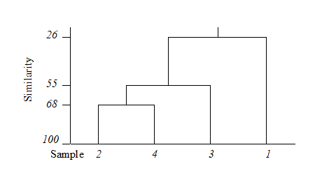
The final merge of all samples into a single group therefore takes place at similarity level 25.9%, and the clustering process for the group-average linking shown in Table 3.2 can be displayed in the following dendrogram.
Dendrogram features
This example raises a number of more general points about the use and appearance of dendrograms.
-
Samples need to be re-ordered along the x axis, for clear presentation of the dendrogram; it is always possible to arrange samples in such an order that none of the dendrogram branches cross each other.
-
The resulting order of samples on the x axis is not unique. A simple analogy would be with an artist’s ‘mobile’; the vertical lines are strings and the horizontal lines rigid bars. When the structure is suspended by the top string, the bars can rotate freely, generating many possible re-arrangements of samples on the x axis. For example, in the above figure, samples 2 and 4 could switch places (new sequence 4, 2, 3, 1) or sample 1 move to the opposite side of the diagram (new sequence 1, 2, 4, 3), but a sequence such as 1, 2, 3, 4 is not possible. It follows that to use the x axis sequence as an ordering of samples is misleading.
-
Cluster analysis attempts to group samples into discrete clusters, not display their inter-relations on a continuous scale; the latter is the province of ordination and this would be preferable for the simple example above. Clustering imposes a rather arbitrary grouping on what appears to be a continuum of change from an unpolluted year (1964), through steadily increasing impact (loss of some species, increase in abundance of opportunists such as Capitella), to the start of a reversion to an improved condition in 1973. Of course it is unwise and unnecessary to attempt serious interpretation of such a small subset of data but, even so, the equivalent MDS ordination for this subset (met in Chapter 5) contrasts well with the relatively unhelpful information in the above dendrogram.
-
The hierarchical nature of this clustering procedure dictates that, once a sample is grouped with others, it will never be separated from them in a later stage of the process. Thus, early borderline decisions which may be somewhat arbitrary are perpetuated through the analysis and may sometimes have a significant effect on the shape of the final dendrogram. For example, similarities S(2, 3) and S(2, 4) above are very nearly equal. Had S(2, 3) been just greater than S(2, 4), rather than the other way round, the final picture would have been a little different. In fact, the reader can verify that had S(1, 4) been around 56% (say), the same marginal shift in the values of S(2, 4) and S(2, 3) would have had radical consequences, the final dendrogram now grouping 2 with 3 and 1 with 4 before these two groups come together in a single cluster. From being the first to be joined, samples 2 and 4 now only link up at the final step. Such situations are certain to arise if, as here, one is trying to force what is essentially a steadily changing pattern into discrete clusters.
Dissimilarities
Exactly the converse operations are needed when clustering from a dissimilarity rather than a similarity matrix. The two samples or groups with the lowest dissimilarity at each stage are fused. The single linkage definition of dissimilarity of two groups is the minimum dissimilarity over all pairs of samples between groups; complete linkage selects the maximum dissimilarity and group-average linking involves just an unweighted mean dissimilarity.
Linkage options
The differing consequences of the three linkage options presented earlier† are most easily seen for the special case used in Chapter 2, where there are only two species (rows) in the original data matrix. Samples are then points in the species space, with the (x,y) axes representing abundances of (Sp.1, Sp.2) respectively. Consider also the case where dissimilarity between two samples is defined simply as their (Euclidean) distance apart in this plot.
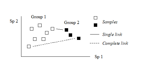
In the above diagram, the single link dissimilarity between Groups 1 and 2 is then simply the minimum distance apart of the two groups, giving rise to an alternative name for the single linkage, namely nearest neighbour clustering. Complete linkage dissimilarity is clearly the maximum distance apart of any two samples in the different groups, namely furthest neighbour clustering. Group-average dissimilarity is the mean distance apart of the two groups, averaging over all between-group pairs.
Single and complete linkage have some attractive theoretical properties. For example, they are effectively non-metric. Suppose that the Bray-Curtis (say) similarities in the original triangular matrix are replaced by their ranks, i.e. the highest similarity is given the value 1, the next highest 2, down to the lowest similarity with rank n(n–1)/2 for n samples. Then a single (or complete) link clustering of the ranked matrix will have the exactly the same structure as that based on the original similarities (though the y axis similarity scale in the dendrogram will be transformed in some non-linear way). This is a desirable feature since the precise similarity values will not often have any direct significance; what matters is their relationship to each other and any non-linear (monotonic) rescaling of the similarities would ideally not affect the analysis. This is also the stance taken for the preferred ordination technique in this manual’s strategy, the method of non-metric multi-dimensional scaling (MDS, see Chapter 5).
However, in practice, single link clustering has a tendency to produce chains of linked samples, with each successive stage just adding another single sample onto a large group. Complete linkage will tend to have the opposite effect, with an emphasis on small clusters at the early stages. (These characteristics can be reproduced by experimenting with the special case above, generating nearest and furthest neighbours in a 2-dimensional species space). Group-averaging, on the other hand, is often found empirically to strike a balance in which a moderate number of medium-sized clusters are produced, and only grouped together at a later stage.
¶ The terminology is inevitably a little confusing therefore! UPGMA is an unweighted mean of the original (dis)similarities among samples but this gives a weighted average among group dissimilarities from the previous merges. Conversely, WPGMA (also known as McQuitty linkage) is defined as an unweighted average of group dissimilarities, leading to a weighted average of the original sample dissimilarities (hence WPGMA).
† PRIMER v7 offers single, complete and group average linking, but also the flexible beta method of Lance & Williams (1967) , in which the dissimilarity of a group (C) to two merged groups (A and B) is defined as $\delta _ {C,AB} = (1 – \beta)[(\delta _ {CA} + \delta _ {CB} ) / 2] + \beta \delta _ {AB} $. If $\beta = 0$ this is WPGMA, $( \delta _ {CA} + \delta _ {CB} ) / 2$, the unweighted average of the two group dissimilarities. Only negative values of $\beta$, in the range (-1, 0), make much sense in theory; Lance and Williams suggest $ \beta = -0.25 $ (for which the flexible beta has affinities with Gower’s median method) but PRIMER computes a range of $ \beta$ values and chooses that which maximises the cophenetic correlation. The latter is a Pearson matrix correlation between original dissimilarity and the (vertical) distance through a dendrogram between the corresponding pair of samples; a dendrogram is a good representation of the dissimilarity matrix if cophenetic correlation is close to 1. Matrix correlation is a concept used in many later chapters, first defined on page 6.10, though there (and usually) with a Spearman rank correlation; however the Pearson matrix correlation is available in PRIMER 7’s RELATE routine, and can be carried out on the cophenetic distance matrix available from CLUSTER. (It is also listed in the results window from a CLUSTER run). In practice, judged on the cophenetic criterion, an optimum flexible beta solution is usually inferior to group average linkage (perhaps as a result of its failure to weight $\delta _ {CA}$ and $\delta _ {CB}$ appropriately when averaging ‘noisy’ data).
3.3 Example: Bristol Channel zooplankton
Collins & Williams (1982) perform hierarchical cluster analyses of zooplankton samples, collected by double oblique net hauls at 57 sites in the Bristol Channel UK, for three different seasons in 1974 {B}. This was not a pollution study but a baseline survey carried out by the Plymouth laboratory, as part of a major programme to understand and model the ecosystem of the estuary. Fig. 3.2 is a map of the sample locations, sites 1-58 (site 30 not sampled).
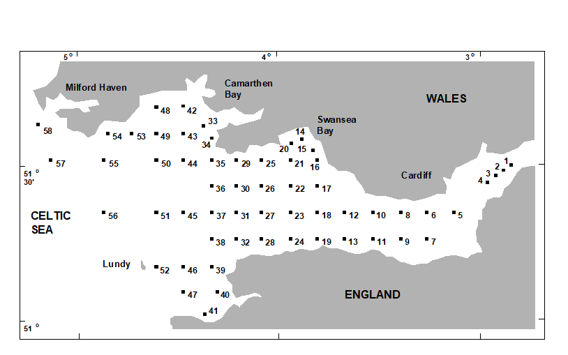 Fig. 3.2 Bristol Channel zooplankton {B}. Sampling sites.
Fig. 3.3 shows the results of a hierarchical clustering using group-average linking of the 57 sites. The raw data were expressed as numbers per cubic metre for each of 24 holozooplankton species, and Bray-Curtis similarities calculated on $\sqrt{}\sqrt{}$-transformed densities. From the resulting dendrogram, Collins and Williams select the four groups determined at a 55% similarity level and characterise these as true estuarine (sites 1-8, 10, 12), estuarine and marine (9, 11, 13-27, 29), euryhaline marine (28, 31, 33-35, 42-44, 47-50, 53-55) and stenohaline marine (32, 36-41, 45, 46, 51, 52, 56-58). A corresponding clustering of species and a re-ordering of the rows and columns of the original data matrix allows the identification of a number of species groups characterising these main site clusters, as is seen later (Chapter 7).
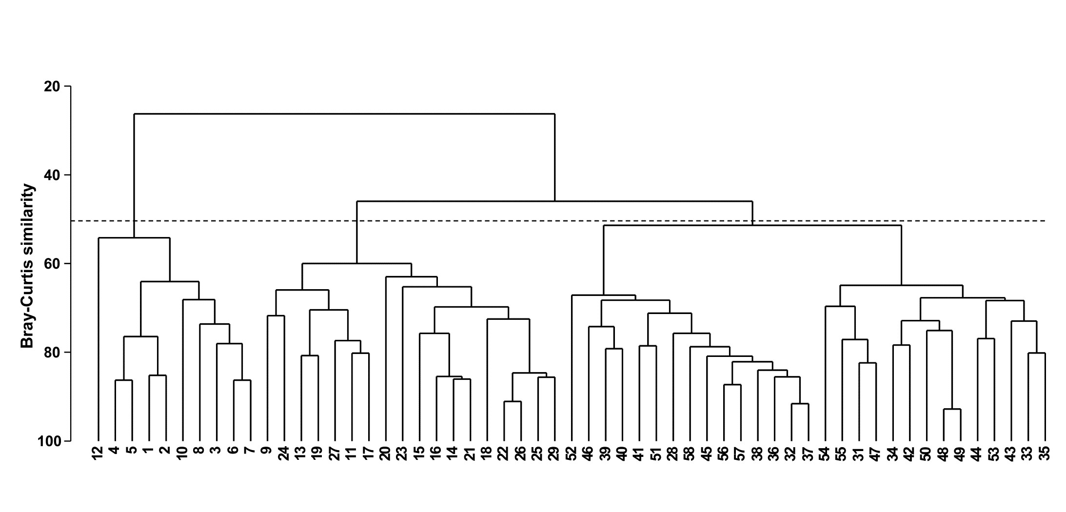
Fig. 3.3. Bristol Channel zooplankton {B}. Dendrogram for hierarchical clustering of the 57 sites, using group-average linking of Bray-Curtis similarities calculated on $\sqrt{}\sqrt{}$-transformed abundance data. The three groups produced by an (arbitrary) threshold similarity of 50% are shown.
The dendrogram provides a sequence of fairly convincing groups; once each of the four main groups has formed it remains separate from other groups over a relatively large drop in similarity. Even so, a cluster analysis gives an incomplete and disjointed picture of the sample pattern. Remembering the analogy of the ‘mobile’, it is not clear from the dendrogram alone whether there is any natural sequence of community change across the four main clusters (implicit in the designations true estuarine, estuarine and marine, euryhaline marine, stenohaline marine). For example, the stenohaline marine group could just as correctly have been rotated to lie between the estuarine and marine and euryhaline marine groups. In fact, there is a strong (and more-or-less continuous) gradient of community change across the region, associated with the changing salinity levels. This is best seen in an ordination of the 57 samples on which are superimposed the salinity levels at each site; this example is therefore returned to in Chapter 11.
3.4 Recommendations
-
Hierarchical clustering with group-average linking, based on sample similarities or dissimilarities such as Bray-Curtis, has proved a useful technique in a number of ecological studies of the past half-century. It is appropriate for delineating groups of sites with distinct community structure (this is not to imply that groups have no species in common, of course, but that different characteristic patterns of abundance are found consistently in different groups).
-
Clustering is less useful (and could sometimes be misleading) where there is a steady gradation in community structure across sites, perhaps in response to strong environmental forcing (e.g. large range of salinity, sediment grain size, depth of water column, etc). Ordination is preferable in these situations.
-
Even for samples which are strongly grouped, cluster analysis is often best used in conjunction with ordination. Superimposition of the clusters (at various levels of similarity) on an ordination plot will allow any relationship between the groups to be more informatively displayed, and it will be seen later (Chapter 5) that agreement between the two representations strengthens belief in the adequacy of both.
-
Historically, in order to define clusters, it was necessary to specify a threshold similarity level (or levels) at which to ‘cut’ the dendrogram (Fig. 3.3 shows a division for a threshold of 50%). This seems arbitrary, and usually is: it is unwise to take the absolute values of similarity too seriously since these vary with standardisation, transformation, taxonomic identification level, choice of coefficient etc. Most of the methods of this manual are a function only of the relative similarities among a set of samples. Nonetheless, it is still an intriguing question to ask how strong the evidence is for the community structure differing between several of the observed groups in a dendrogram. Note the difference between this a posteriori hypothesis and the equivalent a priori test from Fig. 3.1, namely examining the evidence for different communities at (pre-defined) sites A, B, C, etc. A priori groups need the ANOSIM test of Chapter 6; a posteriori ones can be tackled by the similarity profile test (SIMPROF) described below. This test also has an important role in identifying meaningful clusters of species (those which behave in a coherent fashion across samples, see Chapter 7) and in the context of two further (divisive) clustering techniques. The unconstrained form of the latter is described later in this chapter, and its constrained alternative (a linkage tree, ‘explaining’ a biotic clustering by its possible environmental drivers) is in Chapter 11.
3.5 Similarity profiles (SIMPROF)
Given the form of the dendrogram in Fig. 3.3, with high similarities in apparently tightly defined groups and low similarities among groups, there can be little doubt that some genuine clustering of the samples exists for this data set. However, a statistical demonstration of this would be helpful, and it is much less clear, for example, that we have licence to interpret the sub-structure within any of the four apparent main groups. The purpose of the SIMPROF test is thus, for a given set of samples, to test the hypothesis that within that set there is no genuine evidence of multivariate structure (and though SIMPROF is primarily used in clustering contexts, multivariate structure could include seriation of samples, as seen in Chapter 10). Failure to reject this ‘null’ hypothesis debars us from further examination, e.g. for finer-level clusters, and is a useful safeguard to over-interpretation. Thus, here, the SIMPROF test is used successively on the nodes of a dendrogram, from the top downwards.
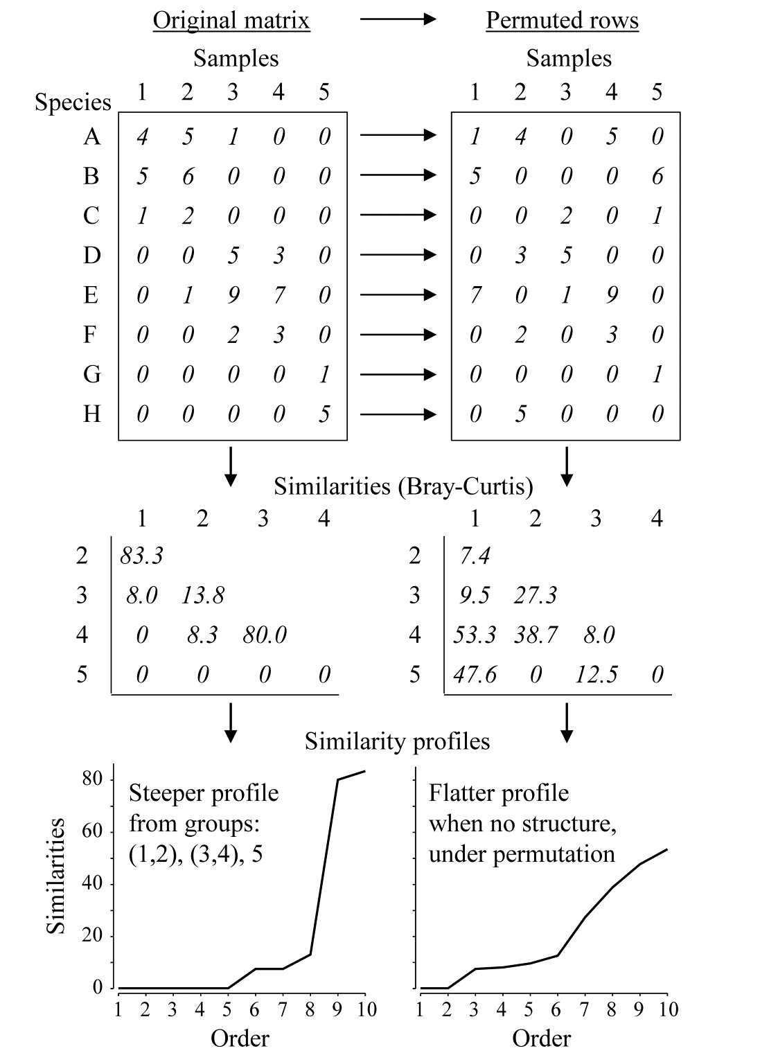 Fig. 3.4. Simple example of construction of a similarity profile from 5 samples (1-5) of 8 species (A-H), for the original matrix (left-hand column) and in a permuted form (right-hand column).
Construction of a single SIMPROF test
The SIMPROF technique is based on the realisation that there is a duality between structure in samples and correlation (association) in species, and Fig. 3.4 demonstrates this for a simple example. The original matrix, in the left-hand column, appears to have a structure of three clusters (samples 1 and 2, samples 3 and 4, and sample 5), driven by, or driving, species sets with high internal associations (A-C, D-F and G-H). This results in some high similarities within the clusters (80, 83.3) and low similarities between the clusters (0, 8, 8.3, 13.8) and few intermediate similarities, in this case none at all. Here, the Bray-Curtis coefficient is used but the argument applies equally to other appropriate resemblance measures. When the triangular similarity matrix is unravelled and the full set of similarities ordered from smallest to largest and plotted on the y axis against that order (the numbers 1, 2, 3, …) on the x axis, a relatively steep similarity profile is therefore obtained (bottom left of Fig. 3.4).
In contrast, when there are no positive or negative associations amongst species, there is no genuinely multivariate structure in the samples and no basis for clustering the samples into groups (or, indeed, identifying other multivariate structures such as gradients of species turnover). This is illustrated in the right-hand column of Fig. 3.4, where the counts for each row of the matrix have been randomly permuted over the 5 samples, independently for each species. There can now be no genuine association amongst species – we have destroyed it by the randomisation – and the similarities in the triangular matrix will now tend to be all rather more intermediate, for example there are no really high similarities and many fewer zeros. This is seen in the corresponding similarity profile which, though it must always increase from left to right, as the similarities are placed in increasing order, is a relatively flatter curve (bottom right, Fig. 3.4).
This illustration suggests the basis for an effective test of multivariate structure within a given group of samples: a schematic of the stages in the SIMPROF permutation test is shown in Fig. 3.5, for a group of 7 samples. The similarity profile for the real matrix needs to be compared with a large set of profiles that would be expected to occur under the null hypothesis that there is no multivariate structure in that group. Examples of the latter are generated by permutation: the independent random re-arrangement of values within rows of the matrix, illustrated once in Fig. 3.4, is repeated (say) 1000 times, each time calculating the full set of similarities and their similarity profile. The bundle of ‘random’ profiles that result are shown in Fig. 3.5 by their mean profile (light, continuous line) and their 99% limits (dashed line). The latter are defined as intervals such that, at each point on the x axis, only 5 of the 1000 permuted profiles fall above, and 5 below, the dashed line. Under the null hypothesis, the real profile (bold line) should appear no different than the other 1000 profiles calculated. Fig. 3.5 illustrates a profile which is not at all in keeping with the randomised profiles and should lead to the null hypothesis being rejected, i.e. providing strong evidence for meaningful clustering (or other multivariate structure) within these 7 samples.
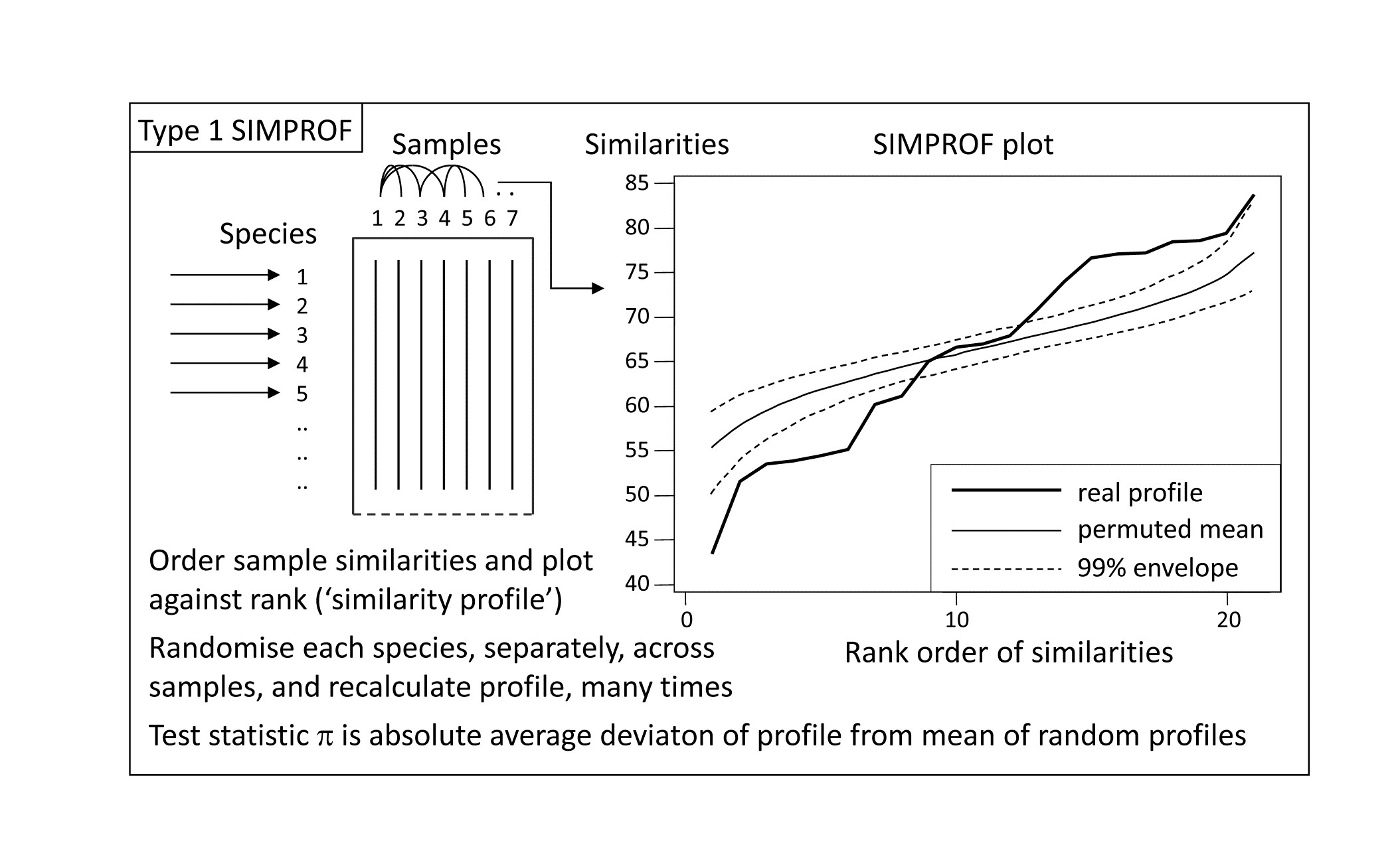 *Fig. 3.5. Schematic diagram of construction of similarity profile (SIMPROF) and testing of null hypothesis of no multivariate structure in a group of samples, by permuting species values. (This is referred to as a Type 1 SIMPROF test, if it needs to be distinguished from Type 2 and 3 tests of species similarities – see Chapter 7. If no Type is mentioned, Type 1 is assumed).
A formal test requires definition of a test statistic and SIMPROF uses the average absolute departure $\pi$ of the real profile from the mean of the permuted ones (i.e. positive and negative deviations are all counted as positive). The null distribution for $\pi$ is created by calculating its value for 999 (say) further random permutations of the original matrix, comparing those random profiles to the mean from the original set of 1000. There are therefore 1000 values of $\pi$, of which 999 represent the null hypothesis conditions and one is for the real profile. If the real $\pi$ is larger than any of the 999 random ones, as would certainly be the case in the schematic of Fig. 3.4, the null hypothesis could be rejected at least at the p < 0.1% significance level. In less clear-cut cases, the % significance level is calculated as 100(t+1)/(T+1)%, where t of the T permuted values of $\pi$ are greater than or equal to the observed $\pi$. For example, if not more than 49 of the 999 randomised values exceed or equal the real $\pi$ then the hypothesis of no structure can be rejected at the 5% level.
SIMPROF for Bristol Channel zooplankton data
Though a SIMPROF test could be used in isolation, e.g. on all samples as justification for starting a multivariate analysis at all, its main use is for a sequence of tests on a hierarchical group structure established by an agglomerative (or divisive) cluster analysis. Using the Bristol Channel zooplankton dendrogram (Fig. 3.3) as an illustration, the first SIMPROF test would be on all 57 sites, to establish that there are at least some interpretable clusters within these. The similarity profile diagram and the resulting histogram of the null distribution for $\pi$ are given in the two left-hand plots of Fig. 3.6. Among the $(57 \times 56)/2 = 1596$ similarities, there are clearly many more large and small, and fewer mid-range ones, than is compatible with a hypothesis of no structure in these samples. (Note that the large number of similarities ensures that the 99% limits hug the mean of the random profiles rather closely.) The real $\pi$ of 6.4 is seen to be so far from the null distribution as to be significant at any specified level, effectively.
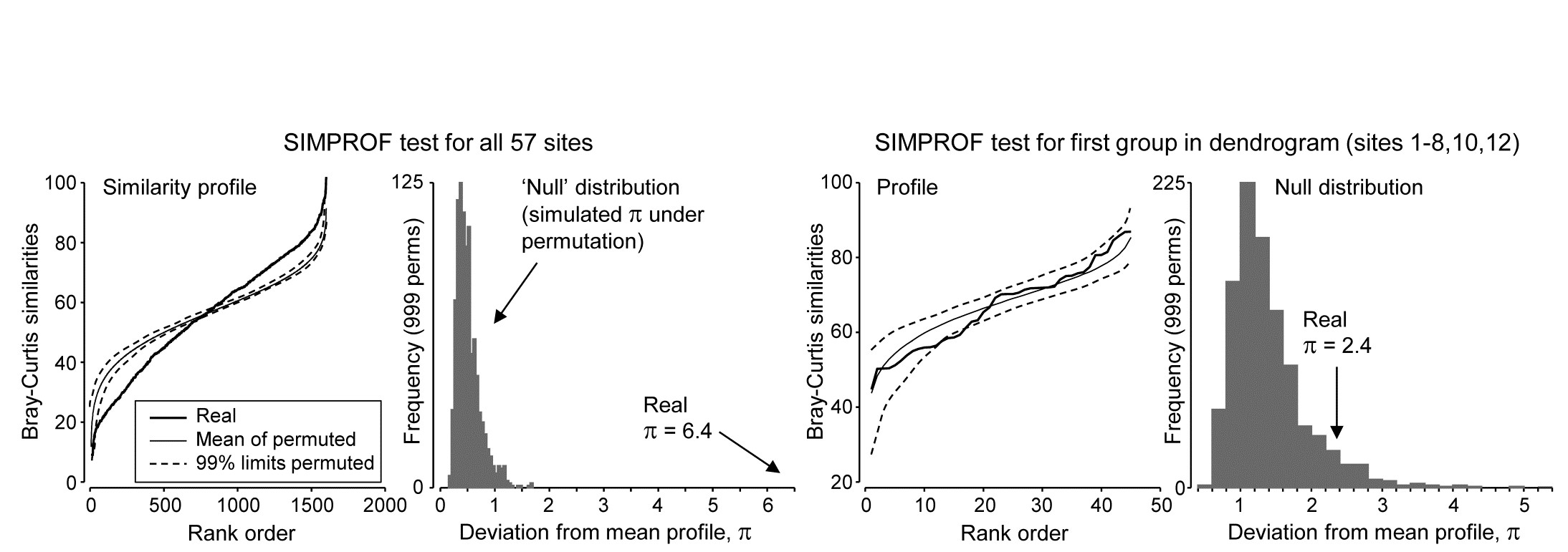
Fig. 3.6. Bristol Channel zooplankton {B}. Similarity profiles and the corresponding histogram for the SIMPROF test, in the case of (left pair) all 57 sites and (right pair) the first group of 10 sites identified in the dendrogram of Fig. 3.3
As is demonstrated in Fig. 3.7, we now drop to the next two levels in the dendrogram. On the left, what evidence is there now for clustering structure within the group of samples {1-8,10,12}? This SIMPROF test is shown in the two right-hand plots of Fig. 3.6: here the real profile lies within the 99% limits over most of its length and, more importantly, the real $\pi$ of 2.4 falls within the null distribution (though in its right tail), giving a significance level p of about 7%. This is marginal, and would not normally be treated as evidence to reject the null hypothesis, especially bearing in mind that multiple significance tests are being carried out.
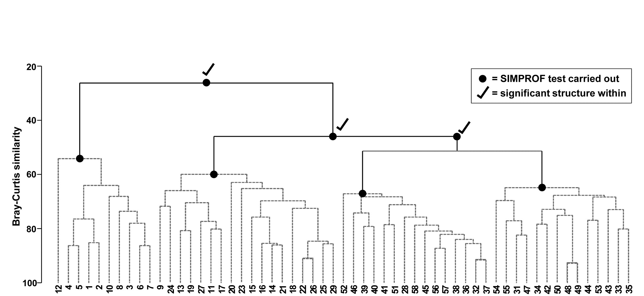
Fig. 3.7. Bristol Channel zooplankton {B}. Dendrogram as in Fig. 3.4 but showing the results of successive SIMPROF tests on nodes of the tree, starting at the top. Only the first three tests showed significant multivariate structure in the samples below that point (bold dots), so there is no evidence from SIMPROF for the detailed clustering structure (grey dashed lines) within each of the 4 main groups.
The conclusion is therefore that there is no clear evidence to allow interpretation of further clusters within the group of samples 1-8,10,12 and this is considered a homogenous set. The remaining 47 samples show strong evidence of heterogeneity in their SIMPROF test (not shown, $\pi = 3.4$, way off the top of the null distribution), so the process drops through to the next level of the dendrogram, where the left-hand group is deemed homogeneous and the right hand group again splits, and so on. The procedure stops quickly in this case, with only four main groups identified as significantly different from each other. The sub-structure of clusters within the four main groups, produced by the hierarchical procedure, therefore has no statistical support and is shown in grey dashed lines in Fig 3.7.
Features of the SIMPROF test
These are discussed more extensively in the primary paper on SIMPROF, Clarke, Somerfield & Gorley (2008) , but some important attributes of the test are worth noting here.
-
A key feature of permutation tests, which are exploited many times in this manual, is that the distribution of abundances (or biomass, area cover etc) for each species remains exactly the same under the random permutations, and is therefore fully realistic. Some species are highly abundant whilst some are much rarer, some species have very right-skewed values, some much less so, and so on. All of this is represented faithfully in the permuted values for each species, since they are exactly the same counts. There is no need to assume specific probability distributions for the test statistics (as in classic statistical tests) or to invoke particular probability distributions for the observations, from which to create matrices simulating the original data (as in Monte Carlo testing). The original data is simply reused, but in a way that is consistent with the null hypothesis being tested. This makes permutation tests, for hypotheses where they can be exploited, extraordinarily general and powerful, as well as simple to understand and interpret.
-
There are at least two asymmetries in the interpretation of a sequence of SIMPROF tests from a cluster hierarchy. Firstly, they provide a ‘stopping rule’ for how far down a dendrogram structure may be interpreted which is not a constant similarity ‘slice’ over the hierarchy: some branches may contain more samples exhibiting more detailed structure, which is validly interpretable at higher similarity levels than other branches. Secondly, in cases where the test sequence justifies interpreting a rather fine-scale group structure (which it would therefore be unwise to interpret at an even more detailed level), it may still be perfectly sensible to choose a coarser sample grouping, by slicing at a lower similarity. SIMPROF gives limits to detailed interpretation but the groups it can identify as differing statistically may be too trivially different to be operationally useful.
-
There can be a good deal of multiple testing in a sequence of SIMPROF tests. Some adjustment for this could be made by Bonferroni corrections. Thus, for the dendrogram of Fig. 3.7, a total of 7 tests are performed. This might suggest repeating the process with individual significance levels of 5/7 = 0.7%, but that is over-precise. What would be informative is to re-run the SIMPROF sequence with a range of significance levels (say 5%, 1%, 0.1%), to see how stable the final grouping is to choice of level. (But scale up your numbers of permutations at higher significance levels, e.g. use at least 9999 for 0.1% level tests; 999 would simply fail to find any significance!). In fact, you are highly likely to find that tinkering with the precise significance levels makes little difference to such a sequence of tests; only a small percentage of the cases will be borderline, the rest being clear-cut in one or other direction. In Fig. 3.7 for example, all four groups are maintained at more stringent significance levels than 5%, until unreasonable levels of 0.01% are reached, when the third and fourth groups (right side of plot) merge.
-
The discussion of more stringent p values naturally raises the issue of power of SIMPROF tests. Power is a difficult concept to formalise in a multivariate context since it requires a precise definition of the alternative to the null hypothesis here of ‘no multivariate structure’, when in fact there are an infinite number of viable alternatives. (These issues are mentioned again in Chapters 6 and 10, and see also Somerfield, Clarke & Olsgard (2002) ). However, in a general sense it is plausible that, all else being equal, SIMPROF will be increasingly likely to detect structure in a group of samples as the group size increases. This is evident if only from the case of just two samples: all random and independent permutations of the species entries over those two samples will lead to exactly the same similarity, hence the real similarity profile (a point) will be at the same position as all the random profiles and could never lead to rejection of the null hypothesis – groups of two are never split. Surprisingly often, though, there is enough evidence to split groups of three into a singleton and pair, an example being for samples 3, 4 and 5 of Fig. 3.4.
-
The number of species will also (and perhaps more clearly) contribute to the power of the test, as can be seen from the obvious fact that if there is just one species, the test has no power at all to identify clusters (or any other structure) among the samples. It does not work by exploring the spacing of samples along a single axis, for example to infer the presence of mixture distributions, a process highly sensitive to distributional assumptions. Instead, it robustly (without such assumptions) exploits associations among species to infer sample structure (as seen in Fig 3.3), and it seems clear that greater numbers of species should give greater power to that inference. It might therefore be thought that adding a rather unimportant (low abundance, low presence) species to the list, highly associated with an existing taxon, will automatically generate significant sample structure, hence of little practical consequence. But that is to miss the subtlety of the SIMPROF test statistic here. It is not constructed from similarities (associations) among species but sample similarities, which will reflect only those species which have sufficient presence or abundance to impact on those similarity calculations (under whatever pre-treatment options of standardising or transforming samples has been chosen as relevant to the context). In other words, for a priori unstructured samples, the test exploits only species associations (either intrinsic or driven by differing environments) that matter to the definition of community patterns, and it is precisely the presence of such associations that define meaningful assemblage structure in that case.
One final point to emphasise. It will be clear to those already familiar with the ANOSIM and RELATE tests of Chapters 6 and 10 that SIMPROF is a very different type of permutation test. ANOSIM starts from a known a priori structure of groups of samples (different sites, times, treatments etc, as in Fig. 3.1), containing replicate samples of each group, and tests for evidence that this imposed group structure is reflected in real differences in similarities calculated among and within groups. If there is such an a priori structure then it is best utilised: though SIMPROF is not invalid in this case, the non-parametric ANOSIM test, or the semi-parametric PERMANOVA test (see the Anderson, Gorley & Clarke (2008) manual) are the correct and better tests. If there is no such prior structuring of samples into groups, and the idea is to provide some rigour to the exploratory nature of cluster analysis, then a sequence of SIMPROF tests is likely to be an appropriate choice: ANOSIM would definitely be invalid in this case. Defining groups by a cluster analysis and then using the same data to test those groups by ANOSIM, as if they were a priori defined, is one of the most heinous crimes in the misuse of PRIMER, occasionally encountered in the literature!
3.6 Binary divisive clustering
All discussion so far has been in terms of hierarchical agglomerative clustering, in which samples start in separate groups and are successively merged until, at some level of similarity, all are considered to belong to a single group. Hierarchical divisive clustering does the converse operation: samples start in a single group and are successively divided into two sub-groups, which may be of quite unequal size, each of those being further sub-divided into two (i.e. binary division), and so on. Ultimately, all samples become singleton groups unless (preferably) some criterion ‘kicks in’ to stop further sub-division of any specific group. Such a stopping rule is provided naturally here by the SIMPROF test: if there is no demonstrable structure within a group, i.e. the null hypothesis for a SIMPROF test cannot be rejected, then that group is not further sub-divided.
Binary divisive methods are thought to be advantageous for some clustering situations: they take a top-down view of the samples, so that the initial binary splits should (in theory) be better able to respect any major groupings in the data, since these are found first (though as with all hierarchical methods, once a sample has been placed within one initial group it cannot jump to another at a later stage). In contrast, agglomerative methods are bottom-up and ‘see’ only the nearby points throughout much of the process; when reaching the top of the dendrogram there is no possibility of taking a different view of the main merged groups that have formed. However, it is not clear that divisive methods will always produce better solutions in practice and there is a counterbalancing downside to their algorithm: it can be computationally more intensive and complex. The agglomerative approach is simple and entirely determined, requiring at each stage (for group average linkage, say) just the calculation of average (dis)similarities between every pair of groups, many of which are known from the previous stage (see the simple example of Table 3.2).
In contrast the divisive approach needs, for each of the current groups, a (binary) flat clustering, a basic idea we meet again below in the context of k-means clustering. That is, we need to look, ideally, at all ways of dividing the n samples of that group into two sub-groups, to determine which is optimal under some criterion. There are $2 ^ {n-1} -1$ possibilities and for even quite modest n (say >25) evaluating all of them quickly becomes prohibitive. This necessitates an iterative search algorithm, using different starting allocations of samples to the two sub-groups, whose members are then re-allocated iteratively until convergence is reached. The ‘best’ of the divisions from the different random restarts is then selected as likely, though not guaranteed, to be the optimal solution. (A similar idea is met in Chapter 5, for MDS solutions.)
The criterion for quantifying a good binary division is clearly central. Classically, ordinary distance (Euclidean) is regarded as the relevant resemblance measure, and Fig. 3.8 (left) shows in 2-d how the total sums of squared distances of all points about the grand mean (overall centroid) is partitioned into a combination of sums of squares within the two groups about their group centroids, and that between the group centroids about the overall centroid (the same principle applies to higher dimensions and more groups). By minimising the within-group sums of squares we maximise that between groups, since the total sums of squares is fixed. For each group, Huygens theorem (e.g. see Anderson, Gorley & Clarke (2008) ) expresses those within-group sums of squares as simply the sum of the squared Euclidean distances between every pair of points in the group (Fig. 3.8, right), divided by that number of points. In other words, the classic criterion minimises a weighted combination of within group resemblances, defined as squared Euclidean distances. Whilst this may be a useful procedure for analysing normalised environmental variables (see Chapter 11), where Euclidean distance (squared) might be a reasonable resemblance choice, for community analyses we need to replace that by Bray-Curtis or other dissimilarities (Chapter 2), and partitioning sums of squares is no longer a possibility. Instead, we need another suitably scaled way of relating dissimilarities between groups to those within groups, which we can maximise by iterative search over different splits of the samples.
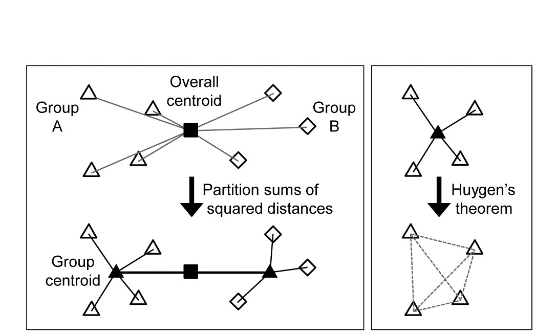
Fig. 3.8. Left: partitioning total sums of squared distances about centroid (d2) into within- and between-group d2. Right: within-group d2 determined by among-point d2, Huygen’s theorem.
There is a simple answer to this, a natural generalisation of the classic approach, met in equation (6.1), where we define the ANOSIM R statistic as:
$$ R = \frac{ \left( \overline{r} _ B - \overline{r} _ W \right) } { \frac{1}{2} M } \tag{3.1} $$
namely the difference between the average of the rank dissimilarities between the (two) groups and within the groups. This is suitably scaled by a divisor of M/2, where M = n(n-1)/2 is the total number of dissimilarities calculated between all the n samples currently being split. This divisor ensures that R takes its maximum value of 1 when the two groups are perfectly separated, defined as all between-group dissimilarities being larger than any within-group ones. R will be approximately zero when there is no separation of groups at all but this will never occur in this context, since we will be choosing the groups to maximise the value of R.
There is an important point not to be missed here: R is in no way being used as a test statistic, the reason for its development in Chapter 6 (for a test of no differences between a priori defined groups, R=0). Instead, we are exploiting its value as a pure measure of separation of groups of points represented by the high-dimensional structure of the resemblances (here perhaps Bray-Curtis, but any coefficient can be used with R, including Euclidean distance). And in that context it has some notable advantages: it provides the universal scaling we need of between vs. within group dissimilarities/distances (whatever their measurement scale) through their reduction to simple ranks, and this non-parametric use of dissimilarities is coherent with other techniques in our approach: non-metric MDS plots, ANOSIM and RELATE tests etc.
To recap: the binary divisive procedure starts with all samples in a single group, and if a SIMPROF test provides evidence that the group has structure which can be further examined, we search for an optimal split of those samples into two groups, maximising R, which could produce anything from splitting off a singleton sample through to an even balance of the sub-group sizes. The SIMPROF test is then repeated for each sub-group and this may justify a further split, again based on maximising R, but now calculated having re-ranked the dissimilarities in that sub-group. The process repeats until SIMPROF cannot justify further binary division on any branch: groups of two are therefore never split (see the earlier discussion).
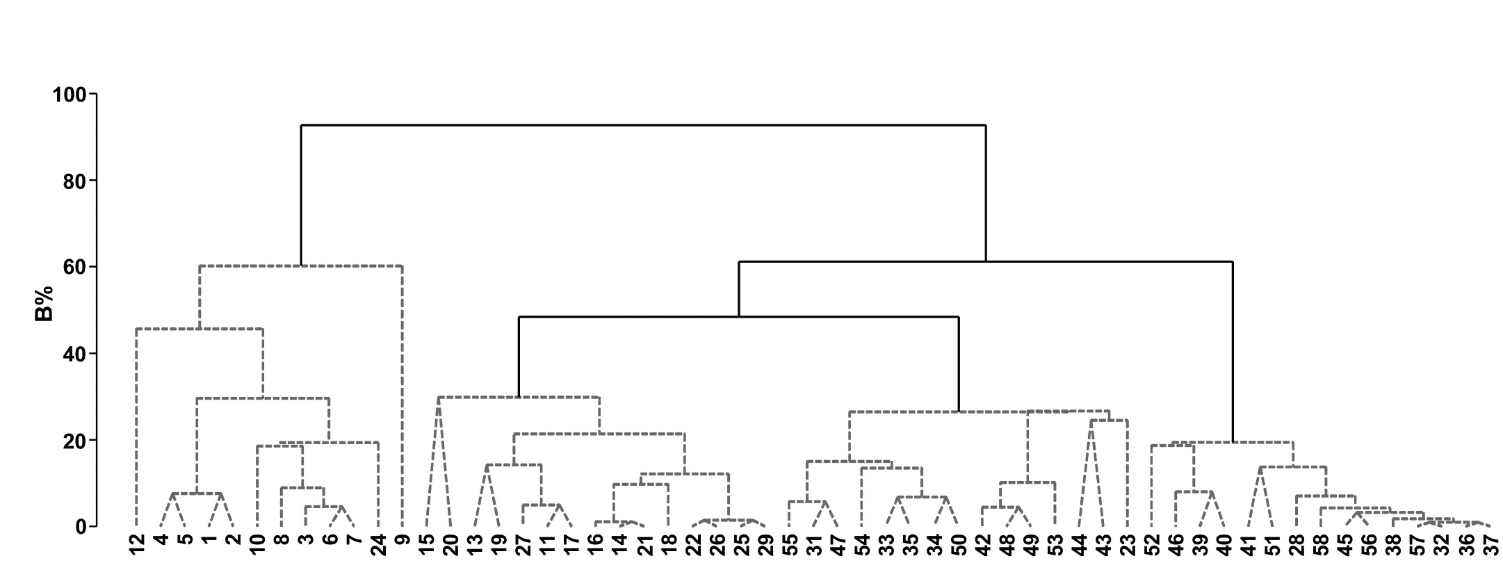
Fig. 3.9. Bristol Channel zooplankton {B}. Unconstrained divisive clustering of 57 sites (PRIMER’s UNCTREE routine, maximising R at each binary split), from Bray-Curtis on $\sqrt{} \sqrt{} $-transformed abundances. As with the agglomerative dendrogram (Fig. 3.7), continuous lines indicate tree structure which is supported by SIMPROF tests; this again divides the data into only four groups.
Bristol Channel zooplankton example
The tree diagram which results from the Bray-Curtis resemblances for the 57 Bristol Channel zooplankton samples is given in Fig 3.9. As with the comparative agglomerative clustering, Fig 3.7, it is convenient to represent all splits down to single points, but the grey dashed lines indicate divisions where SIMPROF provides no support for that sub-structure. Visual comparison of two such trees is not particularly easy, though they have been manually rotated to aid this (remember that a dendrogram is only defined down to arbitrary rotations of its branches, in the manner of a ‘mobile’). Clearly, however, only four groups have been identified by the SIMPROF tests in both cases, and the group constitutions have much in common, though are not identical. This is more readily seen from Figs. 3.10 a & b, which use a non-metric MDS plot (for MDS method see Chapter 5) to represent the community sample relationships in 2-d ordination space. These are identical plots, but demonstrate the agglomerative and divisive clustering results by the use of differing symbols to denote the 4 groups (A-D) produced by the respective trees. The numbering on Fig. 3.10a is that of the sites, shown in Fig. 3.2 (and on Fig. 3.10b the mean salinity at those sites, discretised into salinity scores, see equation 11.2). It is clear that only sites 9, 23 and 24 change groups between the two clustering methods and these all appear at the edges of their groups in both plots, which are thus reassuringly consistent (bear in mind also that a 2-d MDS plot gives only an approximation to the true sample relationships in higher dimensions, the MDS stress of 0.11 here being low but not negligible).
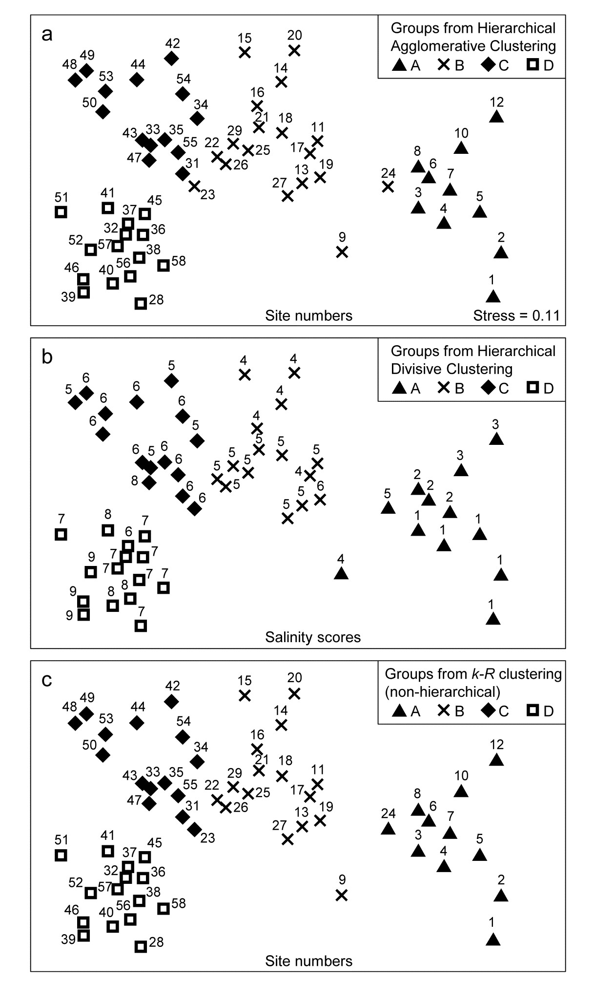
Fig. 3.10. Bristol Channel zooplankton {B}. Non-metric MDS ordination (Chapter 5) of the 57 sites, from Bray-Curtis on $\sqrt{} \sqrt{} $-transformed abundances. Symbols indicate the groups found by SIMPROF tests (four in each case, as it happens) for each of three clustering methods: a) agglomerative hierarchical, b) divisive hierarchical, c) k-R non-hierarchical. Sample labels are: a) & c) site numbers (as in Fig. 3.2), b) site salinity scores (on a 9-point scale, 1: <26.3, …, 9: > 35.1 ppt, see equation 11.2).
PRIMER v7 implements this unconstrained binary divisive clustering in its UNCTREE routine. This terminology reflects a contrast with the PRIMER (v6/ v7) LINKTREE routine for constrained binary divisive clustering, in which the biotic samples are linked to environmental information which is considered to be driving, or at least associated with, the community patterns. Linkage trees, also known as multivariate regression trees, are returned to again in Chapter 11. They perform the same binary divisive clustering of the biotic samples, using the same criterion of optimising R, but the only splits that can be made are those which have an ‘explanation’ in terms of an inequality on one of the environmental variables. Applied to the Bristol Channel zooplankton data, this might involve constraining the splits to those for which all samples in one sub-cluster have a higher salinity score than all samples in the other sub-cluster (better examples for more, and more continuous, environmental variables are given in Chapter 11 and Clarke, Somerfield & Gorley (2008) ). By imposing threshold constraints of this type we greatly reduce the number of possible ways in which splits can be made; evaluation of all possibilities is now viable so an iterative search algorithm is not required. LINKTREE gives an interesting capacity to ‘explain’ any clustering produced, in terms of thresholds on environmental values, but it is clear from Fig. 3.10b that its deterministic approach is quite likely to miss natural clusterings of the data: the C and D groups cannot be split up on the basis of an inequality on the salinity score (e.g. ≤6, ≥7) because this is not obeyed by sites 37 and 47.
For both the unconstrained or constrained forms of divisive clustering, PRIMER offers a choice of y axis scale between equi-spaced steps at each subsequent split (A% scale) and one which attempts to reflect the magnitude of divisions involved (B%), in terms of the generally decreasing dissimilarities between sub-groups as the procedure moves to finer distinctions. Clarke, Somerfield & Gorley (2008) define the B% scale in terms of average between-group ranks based on the originally ranked resemblance matrix, and that is used in Fig. 3.9. The A% scale generally makes for a more easily viewable plot, but the y axis positions at which identifiable groups are initiated cannot be compared.
3.7 k-R clustering (non-hierarchical)
Another major class of clustering techniques is non-hierarchical, referred to above as flat clustering. The desired number of clusters (k) must be specified in advance, and an iterative search attempts to divide the samples in an optimal way into k groups, in one operation rather than incrementally. The classic method, the idea of which was outlined in the two-group case above, is k-means clustering, which seeks to minimise within-group sums of squares about the k group centroids. This is equivalent to minimising some weighted combination of within-group resemblances between pairs of samples, as measured by a squared Euclidean distance coefficient (you can visualise this by adding additional groups to Fig. 3.8). The idea can again be generalised to apply to any resemblance measure, e.g. Bray-Curtis, by maximising ANOSIM R, which measures (non-parametrically) the degree of overall separation of the k groups, formed from the ranks in the full resemblance matrix. (Note that we defined equation (3.1) as if it applied only to two groups, but the definition of R is exactly the same for the k-group case, equation (6.1)). By analogy with k-means clustering, the principle of maximising R to obtain a k-group division of the samples is referred to as k-R clustering, and it will again involve an iterative search, from several different random starting allocations of samples to the k groups.
Experience with k-means clustering suggests that a flat clustering of the k-R type should sometimes have slight advantages over a hierarchical (agglomerative or divisive) method, since samples are able to move between different groups during the iterative process. The k-group solution will not, of course, simply split one of the groups in the (k-1)-group solution: there could be a widescale rearrangement of many of the points into different groups. A widely perceived disadvantage of the k-means idea is the need to specify k before entering the routine, or if it is re-run for many different k values, the absence of a convenient visualisation of the clustering structure for differing values of k, analogous to a dendrogram. This has tended to restrict its use to cases where there is a clear a priori idea of the approximate number of groups required, perhaps for operational reasons (e.g. in a quality classification system). However, the SIMPROF test can also come to the rescue here, to provide a choice of k which is objective. Starting from a low value for k (say 2) the two groups produced by k-R clustering are tested for evidence of within-group structure by SIMPROF. If either of the tests are significant, the routine increments k (to 3), finds the 3-group solution and retests those groups by SIMPROF. The procedure is repeated until a value for k is reached in which none of the k groups generates significance in their SIMPROF test, and the process terminates with that group structure regarded as the best solution. (This will not, in general, correspond to the maximum R when these optima for each k are compared across all possible k; e.g. R must increase to its maximum of 1 as k approaches n, the number of samples.)
Fig. 3.10c shows the optimum grouping produced by k-R clustering, superimposed on the same MDS plot as for Figs. 3.10 a & b. The SIMPROF routine has again terminated the procedure with k=4 groups (A to D), which are very similar to those for the two hierarchical methods, but with the three sites 9, 23 and 24 allocated to the four groups in yet a third way. This appears to be at least as convincing an allocation as for either of the hierarchical plots (though do not lose sight of the fact that the MDS itself is only an approximation to the real inter-sample resemblances).
Average rank form of flat clustering
A variation of this flat-clustering procedure does not use R but a closely related statistic, arising from the concept of group-average linking met earlier in Table 3.2. For a pre-specified number of groups (k), every stage of the iterative process involves removing each sample in turn and then allocating it to one of the k-1 other groups currently defined, or returning it to its original group. In k-R clustering it is re-allocated to the group yielding the highest R for the resulting full set of groups. In the group average rank variation, the sample is re-allocated to the group with which it has greatest (rank) similarity, defined as the average of the pairwise values (from the ranked form of the original similarity matrix) between it and all members of that group – or all of the remaining members, in the case of its original group. The process is iterated until it converges and repeated a fair number of times from different random starting allocations to groups, as before. The choice of k uses the same SIMPROF procedure as previously, and it is interesting to note that, for the Bristol Channel zooplankton data, this group-average variation of k-R clustering produces exactly the same four groups as seen in Fig 3.10c. This will not always be the case because the statistic here is subtly different than the ANOSIM R statistic, but both exploit the same non-parametric form of the resemblance matrix so it should be expected that the two variations will give closer solutions to each other than to the hierarchical methods.
In conclusion
A ‘take-home’ message from Fig. 3.10 is that clustering rarely escapes a degree of arbitrariness: the data simply may not represent clearly separated clusters. For the Bristol Channel sites, where there certainly are plausible groups but within a more or less continuous gradation of change in plankton communities (strongly correlated with increased average salinity of the sites), different methods must be expected to chop this continuum up in slightly different ways. Use of a specific grouping from an agglomerative hierarchy should probably be viewed operationally as little worse (or better) than that from a divisive hierarchy or from the non-hierarchical k-R clustering, in either form; it is reassuring here that SIMPROF supports four very similar groups for all these methods. In fact, especially in cases where a low-dimensional MDS plot is not at all reliable because of high stress (see Chapter 5), the plurality of clustering methods does provide some insight into the robustness of conclusions that can be drawn about group structures from the ‘high-dimensional’ resemblance matrix. Such comparisons of differing clustering methods need to ‘start from the same place’, namely using the same resemblance matrix, otherwise an inferred lack of a stable group structure could be due to the differing assumptions being made about how the (dis)similarity between two samples is defined (e.g. Bray-Curtis vs squared Euclidean distance). This is also a point to bear in mind in the following chapters on competing ordination methods: a primary difference between them is often not the way they choose to represent high-dimensional information in lower dimensional space but how they define that higher-dimensional information differently, in their choice of explicit or implicit resemblance measure.