Chapter 6: Testing for differences between groups of samples
- 6.1 Univariate tests and multivariate tests
- 6.2 ANOSIM for the one-way layout
- 6.3 Example: Frierfjord macrofauna
- 6.4 Example: Indonesian reef-corals
- 6.5 ANOSIM for two-way layouts
- 6.6 Example: Clyde nematodes (2-way nested case)
- 6.7 Example: Eaglehawk Neck meiofauna (two-way crossed case)
- 6.8 Example: Mesocosm experiment (two-way crossed case with no replication)
- 6.9 Example: Exe nematodes (no replication and missing data)
- 6.10 ANOSIM for ordered factors
- 6.11 Example: Ekofisk oil-field macrofauna
- 6.12 Two-way ordered ANOSIM designs
- 6.13 Example: Phuket coral-reef time series
- 6.14 Three-way ANOSIM designs
- 6.15 Example: King Wrasse fish diets, WA
- 6.16 Example: NZ kelp holdfast macrofauna
- 6.17 Example: Tees Bay macrofauna
- 6.18 Recommendations
6.1 Univariate tests and multivariate tests
Many community data sets possess some a priori defined structure within the set of samples, for example there may be replicates from a number of different sites (and/or times). A pre-requisite to interpreting community differences between sites should be a demonstration that there are statistically significant differences to interpret.
Univariate tests
When the species abundance (or biomass) information in a sample is reduced to a single index, such as Shannon diversity (see Chapter 8), the existence of replicate samples from each of the groups (sites/times etc.) allows formal statistical treatment by analysis of variance (ANOVA). This requires the assumption that the univariate index is normally distributed and has constant variance across the groups, conditions which are normally not difficult to justify (perhaps after transformation, see Chapter 9). A so-called global test of the null hypothesis (H$ _ o$), that there are no differences between groups, involves computing a particular ratio of variability in the group means to variability among replicates within each group. The resulting F statistic takes values near 1 if the null hypothesis is true, larger values indicating that H$ _ o$ is false; standard tables of the F distribution yield a significance level (p) for the observed F statistic. Broadly speaking, p is interpreted as the probability that the group means we have observed (or a set of means which appear to differ from each other to an even greater extent) could have occurred if the null hypothesis H$_ o$ is actually true.
Fig.6.1 and Table 6.1 provide an illustration, for the 6 sites and 4 replicates per site of the Frierfjord macrofauna samples. The mean Shannon diversity for the 6 sites is seen in Fig.6.1, and Table 6.1 shows that the F ratio is sufficiently high that the probability of observing means as disparate as this by chance is p<0.001 (or p<0.1%), if the true mean diversity at all sites is the same. This is deemed to be a sufficiently unlikely chance event that the null hypothesis can safely be rejected. Convention dictates that values of p<5% are sufficiently small, in a single test, to discount the possibility that H$_ o$ is true, but there is nothing sacrosanct about this figure: clearly, values of p = 4% and 6% should result in the same inference. It is also clear that repeated significance tests, each of which has (say) a 5% possibility of describing a chance event as a real difference, will cumulatively run a much greater risk of drawing at least one false inference. This is one of the (many) reasons why it is not usually appropriate to handle a multi-species matrix by performing an ANOVA on each species in turn. (Further reasons are the complexities of dependence between species and the general inappropriateness of normality assumptions for abundance-type data).
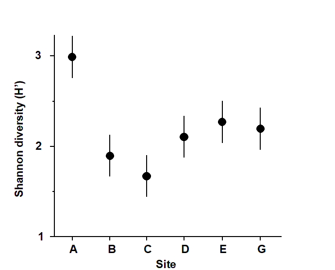
Fig. 6.1. Frierfjord macrofauna {F}. Means and 95% confidence intervals of Shannon diversity (H$^\prime$) at the 6 field sites (A-E, G) shown in Fig. 1.1.
Fig. 6.1 shows the main difference to be a higher diversity at the outer site, A. The intervals displayed are 95% confidence intervals for the true mean diversity at each site; note that these are of equal width because they are based on the assumption of constant variance, that is, they use a pooled estimate of replication variability from the residual mean square in the ANOVA table.
Table 6.1. Frierfjord macrofauna {F}. ANOVA table showing rejection (at a significance level of 0.1%) of the global hypothesis of ‘no site-to-site differences’ in Shannon diversity (H’).
| Sum of squares | Deg. of freedom | Mean Square | F ratio | Sig. level | |
|---|---|---|---|---|---|
| Sites | 3.938 | 5 |
0.788 | 15.1 | < 0.1% |
| Residual | 0.937 | 18 | 0.052 | ||
| Total | 4.874 | 23 |
Further details of how confidence intervals are determined, why the ANOVA F ratio and F tables are defined in the way they are, how one can allow to some extent for the repeated significance tests in pairwise comparisons of site means etc, are not pursued here. This is the ground of basic statistics, covered by many standard texts, for example
Sokal & Rohlf (1981)
, and such computations are available in all general-purpose statistics packages. This is not to imply that these concepts are elementary; in fact it is ironic that a proper understanding of why the univariate F test works requires a level of mathematical sophistication that is not needed for the simple permutation approach to the analogous global test for differences in multivariate structure between groups, outlined below.
Multivariate tests
One important feature of the multivariate analyses described in earlier chapters is that they in no way utilise any known structure among the samples, e.g. their division into replicates within groups. (This is in contrast with Canonical Variate Analysis, for example, which deliberately seeks out ordination axes that, in a certain well-defined sense, best separate out the known groups; e.g. Mardia, Kent & Bibby (1979) ). Thus, the ordination and dendrogram of Fig 6.2, for the Frierfjord macrofauna data, are constructed only from the pairwise similarities among the 24 samples, treated simply as numbers 1 to 24. By superimposing the group (site) labels A to G on the respective replicates it becomes immediately apparent that, for example, the 4 replicates from the outer site (A) are quite different in community composition from both the mid-fjord sites B, C and D and the inner sites E and G. A statistical test of the hypothesis that there are no site-to-site differences overall is clearly unnecessary, though it is less clear whether sufficient evidence exists to assert that B, C and D differ.
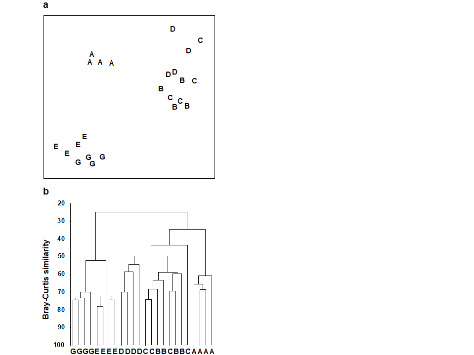
Fig. 6.2 Frierfjord macrofauna {F}. a) MDS plot, b) dendrogram, for 4 replicates from each of the 6 sites (A-E and G), from Bray Curtis similarities computed for $\sqrt{} \sqrt{}$-transformed species abundances (MDS stress = 0.05).
This simple structure of groups, and replicates within groups, is referred to as a 1-way layout, and it was seen above that 1-way ANOVA would provide the appropriate testing framework if the data were univariate (e.g. diversity or total abundance across all species). There is an analogous multivariate analysis of variance (MANOVA, e.g. Mardia, Kent & Bibby (1979) ), in which the F test is replaced by a test known as Wilks’ $\Lambda$, but its assumptions will never be satisfied for typical multi-species abundance (or biomass) data. This is the problem referred to in the earlier chapters on choosing similarities and ordination methods; there are typically many more species (variables) than samples and the probability distribution of counts could never be reduced to approximate (multivariate) normality, by any transformation, because of the dominance of zero values. For example, for the Frierfjord data, as many as 50% of the entries in the species/samples matrix are zero, even after reducing the matrix to only the 30 most abundant species!
A valid test can instead be built on a simple non-parametric permutation procedure, applied to the (rank) similarity matrix underlying the ordination or classification of samples, and therefore termed an ANOSIM test (analysis of similarities)¶, by analogy with the acronym ANOVA (analysis of variance). The history of such permutation tests dates back to the epidemiological work of Mantel (1967) , and this is combined with a general randomization approach to the generation of significance levels ( Hope (1968) ). In the context below, it was described by Clarke & Green (1988) .
¶ The PRIMER ANOSIM routine covers tests for replicates from 1-, 2- and 3-way (nested or crossed) layouts in all combinations. In 2- or 3-way crossed cases without replication, a special form of the ANOSIM routine can still provide a (rather different style of) test; all the possibilities are worked through in this chapter.
6.2 ANOSIM for the one-way layout
Fig.6.3 displays the MDS based only on the 12 samples (4 replicates per site) from the B, C and D sites of the Frierfjord macrofauna data. The null hypothesis (H$_o$) is that there are no differences in community composition at these 3 sites. In order to examine H$_o$, there are 3 main steps:
-
Compute a test statistic reflecting the observed differences between sites, contrasted with differences among replicates within sites. Using the MDS plot of Fig. 6.3, a natural choice might be to calculate the average distance between every pair of replicates within a site, and contrast this with the average distance apart of all pairs of samples corresponding to replicates from different sites. A test could certainly be constructed from these distances but it would have a number of drawbacks.
a) Such a statistic could only apply to a situation in which the method of display was an MDS rather than, say, a cluster analysis.
b) The result would depend on whether the MDS was constructed in two, three or higher dimensions. There is often no ‘correct’ dimensionality and one may end up viewing the picture in several different dimensions – it would be unsatisfactory to generate different test statistics in this way.
c) The configuration of B, C and D replicates in Fig. 6.3 also differs slightly from that in Fig. 6.2a, which includes the full set of sites A-E, G. It is again undesirable that a test statistic for comparing only B, C and D should depend on which other sites are included in the picture.
These three difficulties disappear if the test is based not on distances between samples in an MDS but on the corresponding rank similarities between samples in the underlying triangular similarity matrix. If $\overline{r}_W$ is defined as the average of all rank similarities among replicates within sites, and $\overline{r}_B$ is the average of rank similarities arising from all pairs of replicates between different sites¶, then a suitable test statistic is $$ R = \frac{ \left( \overline{r}_B - \overline{r}_W \right) }{ \frac{1}{2} M} \tag{6.1} $$ where M = n(n–1)/2 and n is the total number of samples under consideration. Note that the highest similarity corresponds to a rank of 1 (the lowest value), following the usual mathematical convention for assigning ranks.
The denominator constant in equation (6.1) has been chosen so that:
a) R can never technically lie outside the range (-1,1);
b) R = 1 only if all replicates within sites are more similar to each other than any replicates from different sites;
c) R is approximately zero if the null hypothesis is true, so that similarities between (among¶) and within sites will be the same on average.
R will usually fall between 0 and 1, indicating some degree of discrimination between the sites. R substantially less than zero is unlikely since it would correspond to similarities across different sites being higher than those within sites; such an occurrence is more likely to indicate an incorrect labelling of samples.† The R statistic itself is a very useful comparative measure of the degree of separation of sites§, and its value is at least as important as its statistical significance, and arguably more so. As with standard univariate tests, it is perfectly possible for R to be significantly different from zero yet inconsequentially small, if there are many replicates at each site.
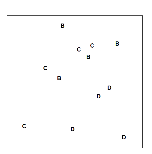
Fig. 6.3. Frierfjord macrofauna {F}. MDS ordination as for Fig. 6.2 but computed only from the similarities involving sites B, C and D (stress = 0.11).
-
Recompute the statistic under permutations of the sample labels. Under the null hypothesis H$ _ o$: ‘no difference between sites’, there will be little effect on average to the value of R if the labels identifying which replicates belong to which sites are arbitrarily rearranged; the 12 samples of Fig. 6.3 are just replicates from a single site if H$ _ o$ is true. This is the rationale for a permutation test of H$ _ o$; all possible allocations of four B, four C and four D labels to the 12 samples are examined and the R statistic recalculated for each. In general there are
$$ \left( kn \right) ! / \left[ \left( n! \right)^k k! \right] \tag{6.2}$$
distinct ways of permuting the labels for n replicates at each of k sites, giving 5775 permutations here. It is computationally possible to examine this number of re-labellings but the scale of calculation can quickly get out of hand with modest increases in replication, so the full set of permutations is randomly sampled (usually with replacement) to give the null distribution of R. In other words, the labels in Fig. 6.3 are randomly reshuffled, R recalculated and the process repeated a large number of times (T).
- Calculate the significance level by referring the observed value of R to its permutation distribution. If H$ _ o$ is true, the likely spread of values of R is given by the random rearrangements, so that if the true value of R looks unlikely to have come from this distribution there is evidence to reject the null hypothesis. Formally (as seen for the earlier SIMPROF test), if only t of the T simulated values of R are as large (or larger than) the observed R then H$_o$ can be rejected at a significance level of (t+1)/(T+1), or in percentage terms, 100(t+1)/(T+1)%.
¶ There is an interesting semantic difference here between US and British English, which has occasionally caused confusion in the literature! Here ‘between groups’ can imply between several groups and not just two (see Fowler’s Modern English Usage) whereas US usage always prefers ‘among groups’ in that context.
† Chapman & Underwood (1999) point out some situations in which negative R values (though not necessarily significantly negative) do occur in practice, when the community is species- poor and individuals have a heavily clustered spatial distribution, so that variability within a group is extreme. It usually also requires a design failure, e.g. a major stratifying factor (a differing substrate, say) is encompassed within each group but its effect is ignored in the analysis.
§ As was seen when assessing relative magnitude of competing group divisions in divisive cluster analysis, in Chapter 3.
6.3 Example: Frierfjord macrofauna
The rank similarities underlying Fig. 6.3 are shown in Table 6.2 (note that these are the similarities involving only sites B, C and D, extracted from the matrix for all sites and re-ranked). Averaging across the 3 diagonal sub-matrices (within groups B, C and D) gives $\overline{r}_W = 22.7$, and across the remaining (off-diagonal) entries gives $\overline{r}_B = 37.5$. Also $n = 12$ and $M = 66$, so that $R = 0.45$. In contrast, the spread of R values possible from random re-labelling of the 12 samples can be seen in the histogram of Fig. 6.4: the largest of $T = 999$ simulations is less than 0.45 ($t = 0$). An observed value of $R = 0.45$ is seen to be a most unlikely event, with a probability of less than 1 in a 1000 if H$_o$ is true, and we can therefore reject H$_o$ at a significance level of p<0.1% (at least, because $R = 0.45$ may still have been the most extreme outcome observed had we chosen an even larger number of permutations. If it is the most extreme of all 5775 – it will be one of them – then p = 100(1/5775) = 0.02%).
Table 6.2. Frierfjord macrofauna {F}. Rank similarity matrix for the 4 replicates from each of B, C and D, i.e. C3 and C4 are the most, and B1 and C1 the least, similar samples.
| B1 | B2 | B3 | B4 | C1 | C2 | C3 | C4 | D1 | D2 | D3 | D4 | |
|---|---|---|---|---|---|---|---|---|---|---|---|---|
| B1 | – | |||||||||||
| B2 | 33 | – | ||||||||||
| B3 | 8 | 7 | – | |||||||||
| B4 | 22 | 11 | 19 | – | ||||||||
| C1 | 66 | 30 | 58 | 65 | – | |||||||
| C2 | 44 | 3 | 15 | 28 | 29 | – | ||||||
| C3 | 23 | 16 | 5 | 38 | 57 | 6 | – | |||||
| C4 | 9 | 34 | 4 | 32 | 61 | 10 | 1 | – | ||||
| D1 | 48 | 17 | 42 | 56 | 37 | 55 | 51 | 62 | – | |||
| D2 | 14 | 20 | 24 | 39 | 52 | 46 | 35 | 36 | 21 | – | ||
| D3 | 59 | 49 | 50 | 64 | 54 | 53 | 63 | 60 | 43 | 41 | – | |
| D4 | 40 | 12 | 18 | 45 | 47 | 27 | 26 | 31 | 25 | 2 | 13 | – |
Pairwise tests
The above is a global test, indicating that there are site differences somewhere that may be worth examining further. Specific pairs of sites can then be compared: for example, the similarities involving only sites B and C are extracted, re-ranked and the test procedure repeated, giving an R value of 0.23. This time there are only 35 distinct relabellings so, under the null hypothesis H$ _ o$ that sites B and C do not differ, the full permutation distribution of possible values of R can be computed; 12% of these values are equal to or larger than 0.23 so H$ _ o$ cannot be rejected. By contrast, R = 0.54 for the comparison of B against D, which is the most extreme value possible under the 35 permutations. B and D are therefore inferred to differ significantly at the p< 3% level. For C against D, R = 0.57 similarly leads to rejection of the null hypothesis (p<3%).
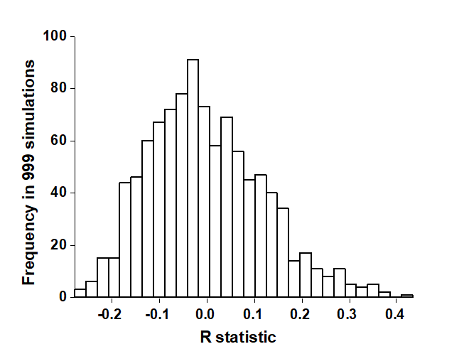
Fig. 6.4. Frierfjord macrofauna {F}. Permutation distribution of the test statistic R (equation 6.1) under the null hypothesis of ‘no site differences’; this contrasts with an observed value for R of 0.45.
There is a danger in such repeated significance tests which should be noted (although rather little can be done to ameliorate it here). To reject the null hypothesis at a significance level of 3% implies that a 3% risk is being run of drawing an incorrect conclusion (a Type I error in statistical terminology). If many such tests are performed this risk will cumulate. For example, all pairwise comparisons between 10 sites, each with 4 replicates (allowing 3% level tests at best), would involve 45 tests, and the overall risk of drawing at least one false conclusion is high. For the analogous pairwise comparisons following the global F test in a univariate ANOVA, there exist multiple comparison tests which attempt to adjust for this repetition of risk. One straightforward possibility, which could be carried over to the present multivariate test, is a Bonferroni correction. In its simplest form, this demands that, if there are n pairwise comparisons in total, each test uses a significance level of 0.05/n. The so-called experiment-wise Type I error, the overall probability of rejecting the null hypothesis at least once in the series of pairwise tests, when there are no genuine differences, is then kept to 0.05.
However, the difficulty with such a Bonferroni correction is clear from the above example: with only 4 replicates in each group, and thus only 35 possible permutations, a significance level of 0.05/3 (=1.7%) can never be achieved! It may be possible to plan for a modest improvement in the number of replicates: 5 replicates from each site would allow a 1% level test for a pairwise comparison, equation (6.2) showing that there are then 126 permutations, and two groups of 6 replicates would give close to a 0.2% level test. However, this may not be realistic in some practical contexts, or it may be inefficient to concentrate effort on too many replicates at one site, rather than (say) increasing the spatial coverage of sites. Also, for a fixed number of replicates, a too demandingly low Type I error (significance level) will be at the expense of a greater risk of Type II error, the probability of not detecting a difference when one genuinely exists.
Strategy for interpretation
The solution, as with all significance tests, is to treat them in a more pragmatic way, exercising due caution in interpretation certainly, but not allowing the formality of a test procedure for pairwise comparisons to interfere with the natural explanation of the group differences. Herein lies the real strength of defining a test statistic, such as R, which has an absolute interpretation of its value†. This is in contrast to a standard Z-type statistic, which typically divides an appropriate measure (taking the value zero under the null hypothesis) by its standard deviation, so that interpretation is limited purely to statistical significance of the departure from zero.
The recommended course of action, for a case such as the above Frierfjord data, is therefore always to carry out, and take totally seriously, the global ANOSIM test for overall differences between groups. Usually the total number of replicates, and thus possible permutations, is relatively large, and the test will be reliable and informative. If it is not significant, then generally no further interpretation is permissible. If it is significant, it is legitimate to ask where the main between-group differences have arisen. The best tool for this is an examination of the R value for each pairwise comparison: large values (close to unity) are indicative of complete separation of the groups, small values (close to zero) imply little or no segregation. If the MDS is of sufficiently low stress to give a reliable picture, then the relative group separations will also be evident from this.¶ The R value itself is not unduly affected by the number of replicates in the two groups being compared; this is in stark contrast to its statistical significance, which is dominated by the group sizes (for large numbers of replicates, R values near zero could still be deemed ‘significant’, and conversely, few replicates could lead to R values close to unity being classed as ‘non-significant’).
The analogue of this approach in the univariate case (say in the comparison of species richness between sites) would be firstly to compute the global F test for the ANOVA. If this establishes that there are significant overall differences between sites, the size of the effects would be ascertained by examining the differences in mean values between each pair of sites, or equivalently, by simply looking at a plot of how the mean richness varies across sites (usually without the replicates also shown). It is then immediately apparent where the main differences lie, and the interpretation is a natural one, emphasising the important biological features (e.g. absolute loss in richness is 5, 10, 20 species, or relative loss is 5%, 10%, 20% of the species pool, etc), rather than putting the emphasis solely on significance levels in pairwise comparisons of means that run the risk of missing the main message altogether.
So, returning to the multivariate data of the above Frierfjord example, interpretation of the ANOSIM tests is seen to be straightforward: a significant level (p<0.1%) and a mid-range value of R (= 0.45) for the global test of sites B, C and D establishes that there are statistically significant differences between these sites. Similarly mid-range values of R (slightly higher, at 0.54 and 0.57) for the B v D and C v D comparisons, contrasted with a much lower value (of 0.27) for B v C, imply that the explanation for the global test result is that D differs from both B and C, but the latter sites are not distinguishable.
The above discussion has raised the issue of Type II error for an ANOSIM permutation test, and the complementary concept, that of the power of the test, namely the probability of detecting a difference between groups when one genuinely exists. Ideas of power are not easily examined for non-parametric procedures of this type, which make no distributional assumptions and for which it is difficult to specify a precise non-null hypothesis. All that can be obviously said in general is that power will improve with increasing replication, and some low levels of replication should be avoided altogether. For example, if comparing only two groups with a 1-way ANOSIM test, based on only 3 replicates for each group, then there are only 10 distinct permutations and a significance level better than 10% could never be attained. A test demanding a significance level of 5% would then have no power to detect a difference between the groups, however large that difference is!
Generality of application
It is evident that few, if any, assumptions are made about the data in constructing the 1-way ANOSIM test, and it is therefore very generally applicable. It is not restricted to Bray-Curtis similarities or even to similarities computed from species abundance data: it could provide a non-parametric alternative to Wilks’ $\Lambda$ test for data which are more nearly multivariate-normally distributed, e.g. for testing whether groups (sites or times) can be distinguished on the basis of their environmental data (see Chapter 11). The latter would involve computing a Euclidean distance matrix between samples (after suitable transformation and normalising of the environmental variables) and entry of this distance matrix to the ANOSIM procedure. Clearly, if multivariate normality assumptions are genuinely justified then the ANOSIM test must lack sensitivity in comparison with standard MANOVA, but this would seem to be more than compensated for by its greater generality.
Note also that there is no restriction to a balanced number of replicates. Some groups could even have only one replicate provided enough replication exists in other groups to generate sufficient permutations for the global test (though there will be a sense in which the power of the test is compromised by a markedly unbalanced design, here as elsewhere). More usefully, note that no assumptions have been made about the variability of within-group replication needing to be similar for all groups. This is seen in the following example, for which the groups in the 1-way layout are not sites but samples from different years at a single site.
† A standard correlation coefficient, r, would be another example, like ANOSIM R, of a statistic which is both a test statistic (for the null hypothesis of absence of correlation, r = 0) and which has an interpretation as an effect size (large r is strong correlation).
¶ But the comparison of ANOSIM R values is the more generally valid approach, e.g. when the two descriptions do not appear to be showing quite the same thing. Calculation of R is in no way dependent on whether the 2-dimensional approximation implicit in an MDS is satisfactory or not, since R is computed from the underlying, full-dimensional similarity matrix.
6.4 Example: Indonesian reef-corals
Warwick, Clarke & Suharsono (1990) examined data from 10 replicate transects across a single coral-reef site in S. Tikus Island, Thousand Islands, Indonesia, for each of the six years 1981, 1983, 1984, 1985, 1987 and 1988. The community data are in the form of % cover of a transect by each of the 75 coral species identified, and the analysis used Bray-Curtis similarities on untransformed data to obtain the MDS of Fig. 6.5. There appears to be a strong change in community pattern between 1981 and 1983 (putatively linked to the 1982/3 El Niño) and this is confirmed by a 1-way ANOSIM test for these two years alone: R = 0.43 (p< 0.1%). Note that, though not really designed for this situation, the test is perfectly valid in the face of greater variability in 1983 than 1981; in fact it is mainly a change in variability rather than location in the MDS plot that distinguishes the 1981 and 1983 groups (a point returned to in Chapter 15).¶ This is in contrast with the standard univariate ANOVA (or multivariate MANOVA) test, which will have no power to detect a variability change; indeed it is invalid without an assumption of approximately equal variances (or variance-covariance matrices) across the groups.

Fig. 6.5. Indonesian reef corals, S. Tikus Island {I}. MDS of % species cover from 10 replicate transects in each of 6 years: 1 = 1981, 3 = 1983 etc (stress = 0.19).
The basic 1-way ANOSIM test can also be extended to cater for more complex sample designs. Firstly we consider the basic types of 2-factor designs (and later move on to look at 3-factor combinations).
¶ Of course it could equally be argued that, as with any portmanteau test, this is a drawback rather than an advantage of ANOSIM. The price for being able to detect changes of different types is arguably a loss of specificity in interpretation, in cases where it is important to ascribe differences solely to a shift in the ‘mean’ community rather than variation changes. The key point here is that ANOSIM tests the hypothesis of no difference among groups in any way, either (multivariate) location or dispersion. It has more power to detect a location shift than a dispersion difference because of its construction, but a sufficiently large change in either between groups can lead to significance – this is very different than the PERMANOVA test which is constructed to be a test only of location, and assumes constant dispersion. An issue for the latter is how sensitive it is to this assumption, and recent simulation work, Anderson & Walsh (2013) , suggests it is not.
6.5 ANOSIM for two-way layouts
Three types of field and laboratory designs are considered here:
a) the 2-way nested case can arise where two levels of spatial replication are involved, e.g. sites are grouped a priori to be representative of two ‘treatment’ categories (control and polluted, say) but there are also replicate samples taken within sites;
b) the 2-way crossed case can arise from studying a fixed set of sites at several times (with replicates at each site/time combination), or from an experimental study in which the same set of ‘treatments’ (e.g. control and impact) are applied at a number of locations (‘blocks’), for example in the different mesocosm basins of a laboratory experiment, or of course many other combinations of two factors;
c) a 2-way crossed case with no replication of each treatment/block combination can also be catered for, to a limited extent, by a different style of permutation test.
The following examples of cases a) and b) are drawn from Clarke (1993) and the two examples of case c) are from Clarke & Warwick (1994) .
6.6 Example: Clyde nematodes (2-way nested case)
Lambshead (1986) analysed meiobenthic communities from three putatively polluted (P) areas of the Firth of Clyde and three control (C) sites, taking three replicate samples at each site (with one exception). The resulting MDS, based on fourth-root transformed abundances of the 113 species in the 16 samples, is given in Fig. 6.6a. The sites are numbered 1 to 3 for both conditions but the numbering is arbitrary – there is nothing in common between P1 and C1 (say). This is what is meant by sites being ‘nested within conditions’. Two hypotheses are then appropriate:
H1: there are no differences among sites within each treatment (control or polluted conditions);
H2: there are no differences between control and polluted conditions.
The approach to H2 might depend on the outcome of testing H1.
H1 can be examined by extending the 1-way ANOSIM test to a constrained randomisation procedure. The presumption under H1 is that there may be a difference between general location of C and P samples in the multivariate space (as approximately viewed in the MDS plot) but within each condition there cannot be any pattern in allocation of replicates to the three sites. Treating the two conditions entirely separately, one therefore has two separate 1-way permutation analyses of exactly the same type as for the Frierfjord macrofauna data (Fig. 6.3). These generate test statistics $R_C$ and $R_P$, computed from equation (6.1), which can be combined to produce an average statistic $\overline{R}$. This can be tested by comparing it with $\overline{R}$ values from all possible permutations of sample labels permitted under the null hypothesis. This does not mean that all 16 sample labels may be arbitrarily permuted; the randomisation is constrained to take place only within the separate conditions: P and C labels may not be switched. Even so, the number of possible permutations is large (around 20,000).
Notice again that the test is not restricted to balanced designs, i.e. those with equal numbers of replicate samples within sites and/or equal numbers of sites within treatments (although lack of balance causes a minor complication in the efficient averaging of $R_C$ and $R_P$, see Clarke (1988) and Clarke (1993) ). Fig. 6.6b displays the results of 999 simulations (constrained relabellings) from the permutation distribution for $\overline{R}$ under the null hypothesis H1. Possible values range from –0.3 to 0.6, though 95% of the values are seen to be <0.27 and 99% are <0.46. The observed $\overline{R}$ of 0.75 therefore provides a strongly significant rejection of hypothesis H1.

Fig. 6.6. Clyde nematodes {Y}. a) MDS of species abundances from three polluted (P1-P3) and three control sites (C1–C3), with three replicate samples at most sites (stress = 0.09). b) Simulated distribution of the test statistic $\overline{R}$ under the hypothesis H1 of ‘no site differences’ within each condition; the observed $\overline{R}$ is 0.75.
H2, which will usually be the more interesting of the two hypotheses, can now be examined. The test of H1 demonstrated that there are, in effect, only three genuine replicates (the sites 1-3) at each of the two conditions (C and P).
This is a 1-way layout, and H2 can be tested by 1-way ANOSIM but one first needs to combine the information from the three original replicates at each site, to define a similarity matrix for the 6 new ‘replicates’. Consistent with the overall strategy that tests should only be dependent on the rank similarities in the original triangular matrix, averages are first taken over the appropriate ranks to obtain a reduced matrix. For example, the similarity between the three P1 and three P2 replicates is defined as the average of the nine inter-group rank similarities; this is placed into the new similarity matrix along with the 14 other averages (C1 with C2, P1 with C1 etc) and all 15 values are then re-ranked; the 1-way ANOSIM then gives R = 0.74. There are only 10 distinct permutations so that, although this is actually the most extreme R value possible in this case, H2 is only able to be rejected at a p<10% significance level.
The other scenario to consider is that the first test fails to reject H1. There are then two possibilities for examining H2:
a) Proceed with the average ranking and re-ranking exactly as above, on the assumption that even if it cannot be proved that there are no differences between sites it would be unwise to assume that this is so; the test may have had rather little power to detect such a difference.
b) Infer from the test of H1 that there are no differences between sites, and treat all replicates as if they were separate sites, e.g. there would be 7 replicates for control and 9 replicates for polluted conditions in a 1-way ANOSIM test applied to the 16 samples in Fig. 6.6a.
Which of these two courses to take is a matter for debate, and the argument here is exactly that of whether “to pool or not to pool” in forming the residual for the analogous univariate 2-way ANOVA. Option b) will certainly have greater power but runs a real risk of being invalid; option a) is the conservative test and it is certainly unwise to design a study with anything other than option a) in mind.¶
¶ Note that the ANOSIM program in the PRIMER package always takes the first of these options, so if the second option is required the resemblance matrix needs to be put through ANOSIM again, this time as a 1-factor design with the combined factor of condition and site (6 levels, C1, C2, C3, P1, P2, P3 and 3 replicates within most of these levels).
6.7 Example: Eaglehawk Neck meiofauna (two-way crossed case)
An example of a two-way crossed design is given in Warwick, Clarke & Gee (1990) and is introduced more fully here in Chapter 12. This is a so-called natural experiment, studying disturbance effects on meiobenthic communities by the continual reworking of sediment by soldier crabs. Two replicate samples were taken from each of four disturbed patches of sediment, and from adjacent undisturbed areas, on a sand flat at Eaglehawk Neck, Tasmania; Fig. 6.7a is a schematic representation of the 16 sample locations. There are two factors: the presence or absence of disturbance by the crabs and the ‘block effect’ of the four different disturbance patches. It might be anticipated that the community will change naturally across the sand flat, from block to block, and it is important to be able to separate this effect from any changes associated with the disturbance itself. There are parallels here with impact studies in which pollutants affect sections of several bays, so that matched control and polluted conditions can be compared against a background of changing community pattern across a wide spatial scale. There are presumed to be replicate samples from each treatment/block combination (the meaning of the term crossed), though balanced numbers are not essential.
For the Eaglehawk Neck data, Fig. 6.7b displays the MDS for the 16 samples (2 treatments $\times$ 4 blocks $\times$ 2 replicates), based on Bray-Curtis similarities from root-transformed abundances of 59 meiofaunal species. The pattern is remarkably clear and a classic analogue of what, in univariate two-way ANOVA, would be called an additive model. The meiobenthic community is seen to change from area to area across the sand flat but also appears to differ consistently between disturbed and undisturbed conditions. A test for the latter sets up a null hypothesis that there are no disturbance effects, allowing for the fact that there may be block effects, and the procedure is then exactly that of the 2-way ANOSIM test for hypothesis H1 of the nested case. For each separate block an R statistic is calculated from equation (6.1), as if for a simple one-way test for a disturbance effect, and the resulting values averaged to give $\overline{R}$. Its permutation distribution under the null hypothesis is generated by examining all simultaneous re-orderings of the four labels (two disturbed, two undisturbed) within each block. There are only three distinct permutations in each block, giving a total of $3^4$ (= 81) combinations overall and the observed value of $\overline{R}$ (= 0.94) is the highest value attained in the 81 permutations. The null hypothesis is therefore rejected at a significance level of just over 1%.
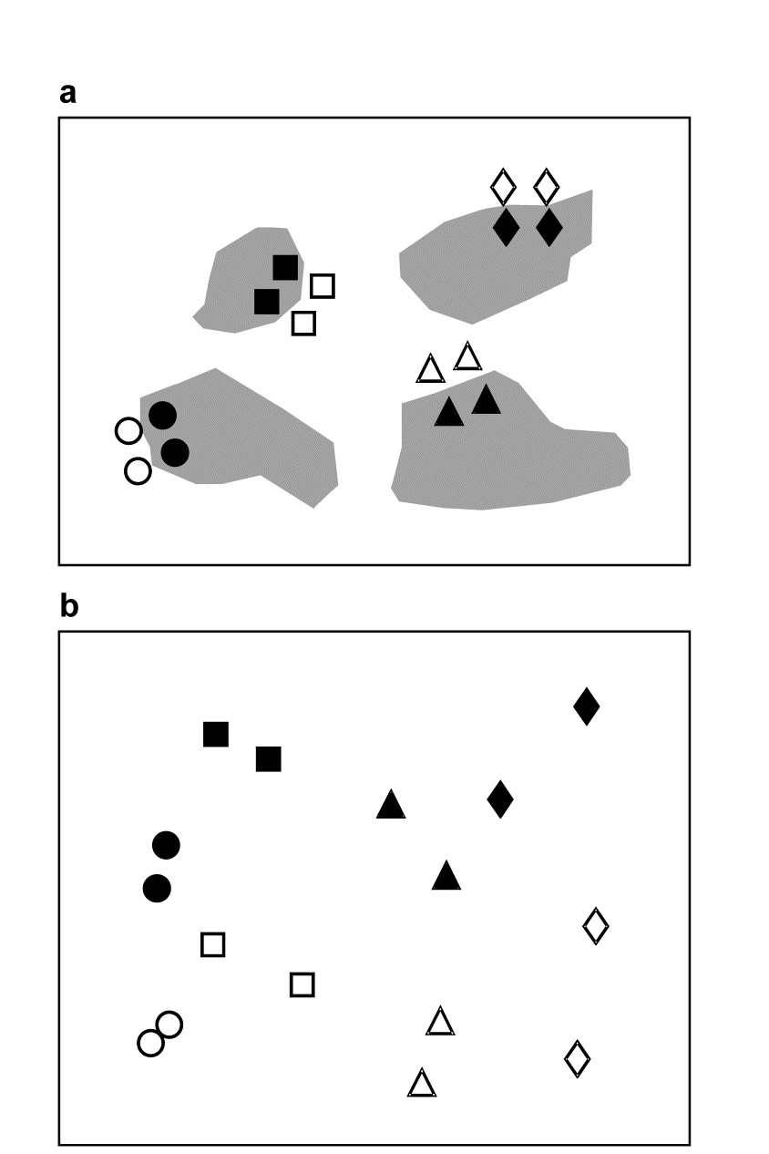
Fig. 6.7. Tasmania, Eaglehawk Neck {T}. a) Schematic of the ‘2-way crossed’ sampling design for 16 meiofaunal cores with two disturbed and two undisturbed replicates from each of four patches of burrowing activity by soldier crabs (shaded). b) MDS of species abundances for the 16 samples, showing separation of the blocks on the x-axis and discrimination of disturbed from undisturbed communities on the y-axis (stress = 0.11).
The procedure departs from the nested case because of the symmetry in the crossed design. One can now test the null hypothesis that there are no block effects, allowing for the fact that there are treatment (disturbance) differences, by simply reversing the roles of treatments and blocks. $\overline{R}$ is now an average of two R statistics, separately calculated for disturbed and undisturbed samples, and there are $8!/[(2!)^4 4!] = 105$ permutations of the 8 labels for each treatment. A random selection from the $105^2 = 11,025$ possible combinations must therefore be made. In 1000 trials the true value of $\overline{R}$ (=0.85) is again the most extreme and is almost certainly the largest in the full set; the null hypothesis is decisively rejected. In this case the test is inherently uninteresting but in other situations (e.g. a sites $\times$ times study) tests for both factors could be of practical importance.
6.8 Example: Mesocosm experiment (two-way crossed case with no replication)
Although the above test may still function if a few random cells in the 2-way layout have only a single replicate, its success depends on reasonable levels of replication overall to generate sufficient permutations. A commonly arising situation in practice, however, is where the 2-way design includes no replication at all.¶ Typically this could be a sites $\times$ times field study (see next section) but it may also occur in experimental work: an example is given by Austen & Warwick (1995) of a laboratory mesocosm study in which a complex array of treatments was applied to soft-sediment cores taken from a single, intertidal location in the Westerschelde estuary, Netherlands, {w}. A total of 64 cores were randomly divided between 4 mesocosm basins, 16 to a basin.
The experiment involved 15 different nutrient enrichment conditions and one control, the treatments being applied to the surface of the undisturbed sediment cores. After 16 weeks controlled exposure in the mesocosm environment, the meiofaunal communities in the 64 cores were identified, and Bray-Curtis similarities on root-transformed abundances gave the MDS of Fig. 6.8. The full set of 16 treatments was repeated in each of the 4 basins (blocks), so the structure is a 2-way treatments $\times$ blocks layout with only one replicate per cell. Little, if any, of this structure is apparent from Fig. 6.8 and a formal test of the null hypothesis
H$_o$: there are no treatment differences (but allowing the possibility of basin effects)
is clearly necessary before any sort of interpretation is attempted.
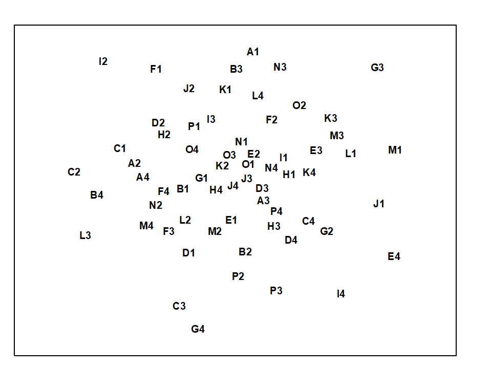
Fig. 6.8. Westerschelde nematodes experiment {w}. MDS of species abundances from 16 different nutrient-enrichment treatments, A to P, applied to sediment cores in each of four mesocosm basins, 1 to 4 (stress = 0.28).
In the absence of replication, a test is still possible in the univariate case, under the assumption that interaction effects are small in relation to the main treatment or block differences ( Scheffe (1959) . In a similar spirit, a global test of H$ _ o$ is possible here, relying on the observation that if certain treatments are responsible for community changes, in a more-or-less consistent way across blocks, separate MDS analyses for each block should show a repeated treatment pattern. This is illustrated schematically in the top half of Fig. 6.9: the fact that treatment A is consistently close to B (and C to D) can only arise if H$_ o$ is false. The analogy with the univariate test is clear: large interaction effects imply that the treatment pattern differs from block to block and there is little chance of identifying a treatment effect; on the other hand, for a treatment $\times$ block design such as the current mesocosm experiment there is no reason to expect treatments to behave very differently in the different basins.
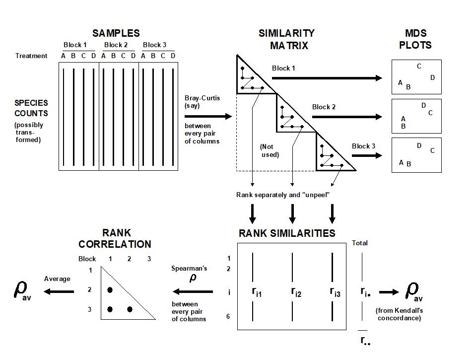 Fig. 6.9. Schematic diagram illustrating the stages in defining concordance of treatment patterns across the blocks, and the two computational routes for$\rho _ {av}$.
What is therefore required is a measure of how well the treatment patterns in the ordinations for the different blocks match; this statistic can then be recomputed under all possible (or a random subset of) permutations of the treatment labels within each block. As previously, if the observed statistic does not fall within the body of this permutation distribution there is significant evidence to reject H$_o$. Note that, as required by the statement of H$_o$, the test makes no assumption about the absence of block effects; between-block similarities are irrelevant to a statistic based only on agreement in within-block patterns.
In fact, for the same reasons advanced for the previous ANOSIM tests (e.g. arbitrariness in choice of MDS dimensionality), it is more satisfactory to define agreement between treatment patterns by reference to the underlying similarity matrix and not the MDS locations. Fig. 6.9 indicates two routes, which lead to equivalent formulations. If there are n treatments and thus N = n(n–1)/2 similarities within a block, a natural choice for agreement of two blocks, j and k, is the Spearman correlation coefficient†
$$ \rho _ {jk} = 1 - \frac {6}{N (N^2 -1)} \sum _ {i=1} ^ N (r_ {ij} - r _ {ik})^2 \tag{6.3} $$
between the matching elements of the two rank similarity matrices {rij, rik; i=1,…,N}, since these ranks are the only information used in successful MDS plots. The coefficients can be averaged across all b(b–1)/2 pairs from the b blocks, to obtain an overall measure of agreement $\rho _ {av}$ on which to base the test. A short cut is to define, from the row totals {$r_ i.$} and grand total $r _{..}$ shown in Fig. 6.9, Kendall's coefficient of concordance ( Kendall (1970) )between the full set of ranks:
$$ W = \frac {12}{b^2 N (N^2 -1)} \sum _ {i=1} ^ N \left( r_ {i.} - \frac{r _ {..}}{N} \right)^2 \tag{6.4} $$
and then exploit the known relationship between this and $\rho _ {av}$:
$$ \rho_{av} = \left( bW - 1 \right) / \left( b - 1 \right) \tag{6.5} $$
As a correlation coefficient, $\rho _ {av}$ takes values in the range (–1, 1), with $ \rho_{av} = 1$ implying perfect agreement and $ \rho_{av} \approx 0$ if the null hypothesis H$_ o$ is true.

Fig. 6.10. Westerschelde nematodes experiment {w}. MDS for the 16 treatments (A to P), performed separately for each of the four basins; no shared treatment pattern is apparent (stress ranges from 0.16 to 0.20).
Note that standard significance tests and confidence intervals for $\rho$ or W (e.g. as given in basic statistical tables) are totally invalid, since they rely on the ranks {$r_{ij}$; i=1,…,N} being from independent variables. This is obviously not true of similarity coefficients from all possible pairs of a set of samples – the samples will be independent but they are repeatedly re-used in calculating the similarities. This does not make $\rho _ {av}$ any the less appropriate, however, as a measure of agreement whose departure from zero (rejection of H$_ o$) is testable by permutation.
For the nutrient enrichment experiment, Fig. 6.10 shows the separate MDS plots for the 4 mesocosm basins. Although the stress values are rather high (and the plots therefore slightly unreliable as a summary of the among treatment relationships), there appears to be no commonality of pattern, and this is borne out by a near zero value for $\rho _ {av}$ of –0.03. This is central to the range of permuted values for $\rho _ {av}$ under H$ _ o$ (obtained by permuting treatment labels separately for each block and recomputing $\rho _ {av}$), so the test provides no evidence of any treatment differences. Note that the symmetry of the 2-way layout also allows a test of the (less interesting) hypothesis that there are no block effects, by looking for any consistency in the among-basin relationships across separate analyses for each of the 16 treatments. The test is again non-significant, with $\rho _ {av} = –0.02$. The negative conclusion to the tests should bar any further attempts at interpretation.
¶ PRIMER 7’s ANOSIM routine automatically switches to attempting the test described here if it finds no replicates to permute. The test will not work for actual or effective 1-way layouts (this is no surprise since univariate ANOVA is powerless to conclude anything if there are no replicates, e.g. in each of 4 treatments it is clearly a silly question to ask: ‘Are the responses 5, 3, 12, 10 different or not?’ if there is no way of assessing the variability in a single number!). But for 2- or 3-factor crossed designs without replication, with enough levels in the tested factor, the test automatically reverts to the correlation method here.
† We will return to this very important concept of a non-parametric matrix (or Mantel) correlation between two resemblance matrices later: it is also at the core of several later Chapters (e.g. 11, 15, 16).
6.9 Example: Exe nematodes (no replication and missing data)
A final example demonstrates a positive outcome to such a test, in a common case of a 2-way layout of sites and times with the additional feature that samples are missing altogether from a small number of cells. Fig. 6.11 shows again the MDS, from Chapter 5, of nematode communities at 19 sites in the Exe estuary.
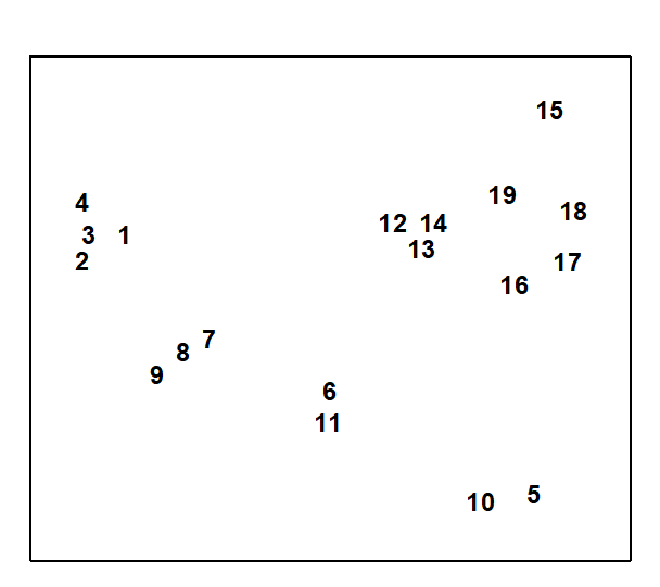
Fig. 6.11. Exe estuary nematodes {X}. MDS, for 19 inter-tidal sites, of species abundances averaged over 6 bi-monthly sampling occasions; see also Fig.5.1 (stress = 0.05).
In fact, this is based on an average of data over six successive bi-monthly sampling occasions. For the individual times, the samples remain strongly clustered into the 4 or 5 main groups apparent from Fig. 6.11. Less clear, however, is whether any structure exists within the largest group (sites 12 to 19) or whether their scatter in Fig. 6.11 is just sampling variation.
Rejection of the null hypothesis of ‘no site differences’ would be suggested by a common site pattern in the separate MDS plots for the 6 times (Fig. 6.12). At some of the times, however, one of the site samples is missing (site 19 at times 1 and 2, site 15 at time 4 and site 18 at time 6). Instead of removing these sites from all plots, in order to achieve matching sets of similarities, one can remove for each pair of times only those sites missing for either of that pair, and compute the Spearman correlation $\rho$ between the remaining rank similarities. The $\rho$ values for all pairs of times are then averaged to give $\rho_{av}$, i.e. the left-hand route is taken in the lower half of Fig. 6.9. This is usually referred to as pairwise removal of missing data, in contrast to the listwise removal that would be needed for the right-hand route. Though increasing the computation time, pairwise removal clearly utilises more of the available information.
Fig. 6.12 shows evidence of a consistent site pattern, for example in the proximity of sites 12 to 14 and the tendency of site 15 to be placed on its own; the fact that site 15 is missing on one occasion does not undermine this perceived structure. Pairwise computation gives $\rho _ {av} = 0.36$ and its significance can be determined by a permutation test, as before. The (non-missing) site labels are permuted amongst the available samples, separately for each time, and these designations fixed whilst all the paired $\rho$ values are computed (using pairwise removal) and averaged. Here the, largest such $\rho _ {av}$ value in 999 simulations was 0.30, so the null hypothesis is rejected at the p<0.1% level.
In the same way, one can also carry out a test of the hypothesis that there are no differences across time for sites 12 to 19. The component plots, of the 4 to 6 times for each site, display no obvious features and $\rho_{av}$= 0.08 (p<18%). The failure to reject this null hypothesis justifies the use of averaged data across the 6 times, in the earlier analyses, and could even be thought to justify use of times as ‘replicates’ for sites in a 1-way ANOSIM test for sites.
Tests of this form, searching for agreement between two or more similarity matrices, occur also in Chapter 11 (in the context of matching species to environmental data) and Chapter 15 (where they link biotic patterns to some model structure). The discussion there includes use of measures other than a simple Spearman coefficient, for example a weighted Spearman coefficient $\rho _ w$ (suggested for reasons explained in Chapter 11), and these adjustments could certainly be implemented here also if desired, using the left-hand route in the lower half of Fig.6.9. In the present context, this type of ‘matching’ test is clearly an inferior one to that possible where genuine replication exists within the 2-way layout. It cannot cope with follow-up tests for differences between specific pairs of treatments, and it can have little sensitivity if the numbers of treatments and blocks are both small. A test for two treatments is impossible note, since the treatment pattern in all blocks would be identical.
Fig. 6.12. Exe estuary nematodes {X}. MDS for sites 12 to 19 only, performed separately for the 6 sampling times (read across rows for time order); in spite of the occasional missing sample some commonality of site pattern is apparent (stress ranges from 0.01 to 0.08).
6.10 ANOSIM for ordered factors
Generalised ANOSIM statistic for the 1-way case
Now return to the simple one-way case of page 6.2, with multivariate data from a number of pre-specified groups (A, B, C, …, e.g. sites, times or treatments) and with replicate samples from each group. It is well known that the ANOSIM test, using the R statistic of equation 6.1, is formally equivalent to a non-parametric Mantel-type test (which PRIMER calls a RELATE test), in which the dissimilarities are correlated with a simple model matrix, using a Spearman rank correlation coefficient ($\rho$, introduced in equation 6.3). Such model matrices are idealised distance matrices which describe the structure expected under the alternative hypothesis (to the null hypothesis of ‘no differences between groups’), and a range of such models are introduced and discussed in Chapter 15, but here we need just the simple case in which samples in the same group are considered to be a distance 0 apart and in different groups a distance 1 unit apart. (The units are not important because Pearson correlation between matching elements is calculated having first ranked both matrices, which is the definition of a Spearman rank correlation).
A RELATE $\rho$ statistic is not the same as an ANOSIM R statistic but the tests (which permute the labels over samples in the same way for the two tests) produce results which are identical because the two statistics are linked, in this simple case, by the relationship:
$$ R = \rho \sqrt{ \frac{ M^2 -1}{3w (M-w)}} \tag{6.6} $$
where w is the number of within-group ranks and M is the total number of ranks in the triangular matrix (thus for the simple example above, with groups A, B, C having replicates 2, 3, 2 respectively, w = 5, M = 21 and R = 1.35 $\rho$).
Importantly, there is a more fundamental relationship between the two statistics, which allows us to generalise the concept of an ANOSIM statistic to cater for ordered models. Then, the test is not of the null:
$$H_0: A = B = C = \ldots $$
against the general alternative
$$H_1: A, B, C, \ldots \text{ differ (in ways unspecified)}$$
but of the same null $H_0$ against an ordered alternative:
$$H_1: A < B < C < \ldots, $$
i.e. A & B and B & C are only one step apart but A & C are 2 steps (and A & D are 3 steps etc). This is an appropriate model for testing, say, for an inter-annual drift in an assemblage away from its initial state, or for serial change in community composition along an environmental gradient (e.g. with increasing water depth or away from a pollution source). The model matrix is now of the form:
and the RELATE test is again the correlation $\rho$ of the dissimilarity ranks {$r_i$} against model ranks {$s_i$}. In contrast, the generalised ANOSIM statistic is defined totally generally as the slope of a linear regression of {$r_i$} on {$s_i$}, and denoted in the above ordered case by $R^O$ (the superscript upper case O denoting ‘ordered’). Testing of this statistic uses the appropriate permutation distribution; standard tests (or interval estimates) for the slope of the regression cannot be used because of the high degree of internal dependency among the {$r_i$} (dissimilarities are not mutually independent).
Several important points follow from this definition. Firstly, it takes only a few lines of algebra to show that, in the unordered case, this slope reduces to the usual ANOSIM R statistic. Secondly, the equations defining slopes and correlations dictate that $R^O$ is zero if and only if $\rho$ is zero, the null hypothesis condition. Thirdly, $R^O$ can never exceed 1 and it takes that value only under a generalisation of our standard ‘mantra’ for the (non-parametrically) most extreme multivariate separation that can be observed between groups, namely that ‘all dissimilarities between groups are larger than any within groups’, to which we must now add ‘and all dissimilarities between groups which are further apart in the model matrix are larger than any dissimilarities between groups which the model puts closer together’. This extreme case is illustrated by the following scatter plot for of {$r_i$} against {$s_i$} for the example above of three ordered groups A< B<C.

The absence of any overlap (or equality) of values on the y axis (for $r_i$) across the three possible tied ranks on the x axis ($s_i$ values) is what ensures that $R^O = 1$.
Fourthly, the model values {$s_i$} will always involve tied ranks in designs with replication (and also for simple trend models without replication), and the plot makes it clear that the correlation $\rho$ cannot in general attain its theoretical maximum of 1 (in all except pathological cases there has to be a scatter of y values at some x axis points). This makes $R^O$ potentially a more useful descriptor for these seriation with replication designs (as they are termed in Chapter 15, and Somerfield, Clarke & Olsgard (2002) ). Finally, one should note the asymmetry of the $R^O$ statistic relative to the symmetry of $\rho$. The generalised ANOSIM concept is restricted to regressing real data in the ranks {$r_i$} on modelled distances in the ranks {$s_i$}; it does not make sense to carry out the regression the other way round. The RELATE $\rho$ statistic, on the other hand, is appropriate for a wider sweep of problems where the interest is in comparing the sample patterns of any two triangular matrices¶; we have already met it used in this way, entirely symmetrically, in equation 6.3, and will do so repeatedly in later chapters.
¶ This contrast is also in part an issue of what to do about tied ranks, and identifies a context-dependent dichotomy noted early in the development of non-parametric methods ( Kendall (1970) ). Would we say that two judges were in perfect agreement only if they ranked 10 candidates in exactly the same order, or does placing the candidates into the same two groups of 5 ‘acceptable’ and 5 ‘not acceptable’ count as perfect agreement? In our case, $\rho$ (the former, which does not adjust for tied ranks) will be more appropriate for some problems, and generalised R (the latter, which does, in effect, build in an adjustment for ties in the {$s_i$}) more appropriate for other problems.
6.11 Example: Ekofisk oil-field macrofauna
Gray, Clarke, Warwick et al. (1990) studied the soft-sediment macrobenthos at 39 sites at different distances (100m to 8km) and different directions away from the Ekofisk oil platform in the N Sea {E}, to examine evidence for changes in the assemblage with distance from the oil-rig. The sites were allocated (somewhat arbitrarily, but a priori) into 4 distance groups, A: >3.5km from the rig (11 sites), B: 1-3.5km (12), C: 250m-1km (10), D: <250m (6). An ordered 1-way ANOSIM test, with sites used as replicates for the four distance groups, does seem preferable here to the standard (unordered) ANOSIM. Though the null hypothesis $H_0: A=B=C=D$ is the same, the ordered alternative $H_1: A<B<C<D$ is an appropriate model for directed community change with distance. That is, there is no need for the test to have power to detect an (uninterpretable) alternative in which, for example, the communities in D are very different from C and B but then very similar to A, so by restricting the alternative to a smaller set of possibilities, we choose to employ a more powerful¶ test statistic $R^O$ for detecting that alternative, and for appropriately measuring its magnitude.
Fig 6.13a shows the (n)MDS for the 39 sites based on square-root transformed abundances of 173 species, under Bray-Curtis dissimilarity, with the 4 distance groups (differing symbols) clearly showing a pattern of steady community change with distance from the oil-rig. Fig 6.13b plots† the $39 \times 38/2 = 741$ rank dissimilarities {$r_i$} against the (ordered) model ranks {$s_i$}, the four sets of tied ranks for the latter representing (left to right): within A, B, C or D; then A to B, B to C or C to D; then A to C or B to D; and finally A to D. The fitted regression of r on s has a strong slope of $R^O = 0.656$, the ordered ANOSIM statistic, and this is larger than its value for 9999 random permutations of the group labels to the 39 samples, so P<0.01% at least (and it would clearly be more significant than effectively any proposed significance boundary here). The contrast is with a standard (unordered) ANOSIM test which records the lower (though still highly significant) value of R = 0.54. Clearly, if there are only two groups, $R^O$ and R become the same statistic, so the pairwise tests between all pairs of groups which follows this (global) ordered ANOSIM test are all exactly the same as for the usual unordered analysis.
 Fig. 6.13. Ekofisk oil-field macrofauna {E}. a) nMDS of the 39 sites from square-root transformed abundances of 173 species and Bray-Curtis similarities, with the four distance groups from the oil-rig indicated by differing symbols. b) Scatter plot of rank dissimilarities (r) among the 39 sites against tied ranks (s) from a serial ordering model of groups, showing the fitted regression line with slope $R^O$, the ordered ANOSIM statistic.
For the four Ekofisk distance groups, the pairwise R values do show the pattern expected from a gradient of change: for groups one step apart (A to B, B to C, C to D), R = 0.56, 0.16, 0.55; for two steps (A to C, B to D), R = 0.76, 0.82; and for three steps (A to D), R = 0.93 (all ‘significant’ by conventional criteria).
Fig. 6.13b clearly demonstrates how the (global) $R^O$ captures both the standard ANOSIM R’s contrast of within and between group ranks (the left-hand set of points vs the right-hand three sets) and the regression relation of greater change with greater distance (the right-hand three). It is thus useful in what follows to distinguish two cases for the ordered 1-way ANOSIM test, namely ordered category and ordered single statistics, denoted by $R^{Oc}$ and $R^{Os}$. The difference is simply that the notation $R^{Oc}$ is used when the data has replicates, so that it gives both a test for the presence of group structure and the ordering of those groups, whereas $R^{Os}$ refers to 1-way layouts with no replicates and where the test is thus entirely based on whether or not there is a serial ordering (trend) in the multivariate pattern of the ‘groups’ (i.e. single samples in this case), in the specified order. Technically, the computation is no different: both are simply the slope of the regression of the ranks {$r_i$} on {$s_i$}, though clearly the unreplicated design requires a reasonable number of ‘groups’ (at least 5, in the 1-way case) to generate sufficient permutations to have any prospect of demonstrating serial change.
¶ Somerfield, Clarke & Olsgard (2002) discuss the difficult issue of power in the context of multivariate analyses (for which a myriad of simple hypotheses make up the complex alternative to ‘no change’, since every species may respond in a different way to potential changes in its environment). They use the Spearman $\rho$ statistic throughout and demonstrate improved power for the alternative ‘seriation with replication’ model over the unordered case.
† Construction of such scatter plots (though not the regression line) can be achieved by a combination of routines on the Tools menu for PRIMER7, i.e. the Ranked resemblance matrix and Ranked triangular matrix created by the Model Matrix option under Seriation are Unravelled and then Merged, to give (x, y) columns for the Scatter Plot. The test itself uses the PRIMER7 extended ANOSIM routine.
6.12 Two-way ordered ANOSIM designs
Under the non-parametric framework adopted in this manual (and in the PRIMER package) three forms of 2-way ANOSIM tests were presented on page 6.5: 2-factor nested, B within A (denoted by B(A)); 2-factor crossed (denoted A$\times$B); and a special case of A$\times$B in which there are no replicates, either because only one sample was taken for each combination of A and B, or replicates were taken but considered to be ‘pseudo-replicates’ (sensu Hurlbert (1984) ) and averaged.¶
The principle of these tests, and their permutation procedures, remain largely unchanged when A or B (or both factors) are ordered. Previously, the test for B under the nested B(A) model (page 6.6) averaged the 1-way $R$ statistic for each level of A, denoted $\overline{R}$, and the same form of averaged statistic was used for testing B under the crossed A$\times$B model with replicates (page 6.7); without replicates the crossed test used the special (and less powerful) construction of page 6.8, with test statistic the pairwise averaged matrix correlation, $\rho_{av}$. (There was no test for B in the nested model, in the absence of replicates for B). If B is now ordered, $R$ is replaced by $R^{Oc}$ where there are replicates (becoming $\overline{R}^{Oc}$ when averaged across the levels of A), or by $R^{Os}$ where there are not (becoming $\overline{R}^{Os}$); there is no longer any necessity to invoke the special form of test based on $\rho_{av}$ when the factor is ordered. The same substitutions then happen for the test of A, if it too is ordered: $\overline{R}$ and $\rho_{av}$ are replaced by $\overline{R}^{Oc}$ and $\overline{R}^{Os}$. If A is not ordered, any ordering in B does not change the way the tests for A are carried out, e.g. for A$\times$B, the A test is still constructed by calculating the appropriate 1-way statistic for A, separately for each level of B, and then averaging those statistics.

Such a plethora of possibilities are best summarised in a table, and the later Table 6.3 lists all the possible combinations of 2-way design, factor ordering (or not) and presence (or absence) of replicates, giving the test statistic and its method of construction, listing whether or not pairwise tests make sense†, and then giving some examples of marine studies in which the factors would have the right structure for such a test.
We have already seen unordered examples of 1-way tests (1a, Table 6.3) in Figs. 6.3 & 6.5, 2-way crossed (2a) in Fig. 6.7 and, without replication (2b), in Figs. 6.10 & 6.12; Fig. 6.6 is 2-way nested (2g). Examples of 2-way crossed without replicates, with one (2d) or both (2f) factors ordered, now follow.
¶ An example of the latter might be ‘replicate’ cores from a multi-corer deployed only once at each of a number of sites (A) for the same set of months (B); these multiple cores are neither spatially representative of the extent of a site (a return trip would result in multi-cores from a slightly different area within the site) nor, it might be argued, temporally representative of that month.
† If they do make sense, the PRIMER7 ANOSIM routine will give them. Performing such a 2-(or 3-) way analysis is much simpler than reading these tables! It is simply a matter of selecting the form of design (all likely combinations of 1-, 2- or 3-factor, crossed or nested) and then specifying which factors are to be considered ordered – the factor levels must be numeric in that case but only their rank order is used. Analyses that use specific numerical levels (unequally-spaced) can be catered for in many cases within the expanded RELATE routine, utilising a $\rho$ statistic, see Chapter 15.
6.13 Example: Phuket coral-reef time series
These data are discussed more fully in Chapters 15 and 16; sampling of coral assemblages took place over a number of years between 1983 and 2000, see Brown, Clarke & Warwick (2002) , along three permanent transects. Transect A, considered here, was sampled on each occasion by twelve ‘10m plotless line samples’, perpendicular to the main transect and spaced at about 10m. Percentage cover of each line sample by each of 53 coral taxa was recorded, {K}.
For this example, we consider a sequence of 7 years of ‘normal’ conditions, i.e. all samples collected over 1988 to 1997 (later chapters examine earlier and later years subject to impacts of different types). This is therefore a two-factor unreplicated crossed design, with one spatial factor (position on transect) and one temporal factor (year), with the spatial factor clearly ordered and the temporal factor capable of being analysed either as unordered or ordered, depending on whether the test is for non-specific inter-annual variation or for a trend in time.
Fig. 6.14 shows the MDS of the beginning and ending years of this selected time period, for the 12 positions along the transect (inshore to offshore, 1 to 12), based on Bray-Curtis similarities from the root-transformed %cover data. The other 4 years have similarly clear spatial trends, so it is not surprising that the ordered ANOSIM test for Position (the B factor in case 2d of Table 6.3), which uses the unreplicated $\overline{R}^{Os}$ statistic, an average of the separate $R^{Os}$ statistics over 7 years, returns the high value of 0.68 (p < 0.1%, though significant at any specified level, in practice). In spite of the absence of replication, separate analyses of the position factor for each year are now possible, i.e. a 1-way ordered ANOSIM without replication (case 1d). E.g. the spatial trends seen in Fig. 6.14 for 1988 and 1997 have $R^{Os} = 0.65$ and 0.73 (both p < 0.1%).
Fig. 6.14. Ko Phuket corals {K}. nMDS for two years from coral cover of 53 taxa (root-transform, Bray-Curtis similarities), at 12 positions along an inshore-offshore transect.
The general test for the Year factor (A in case 2d of Table 6.3), in contrast gives $\rho_{av} = 0.02$ (ns, no year effect). A more directed test of a trend over the seven years between the starting and ending configurations seen in Fig. 6.14 (case 2f), based on an average of the $R^{Os}$ statistics through the years, separately for each transect position, also gives a low and non-significant value for $\overline{R}^{Os}$ of 0.08 (p $\approx$ 10%). However, if earlier and later years are also included, which saw a sedimentation impact and a prolonged desiccation of the reefs, then a small trend is detected $\overline{R}^{Os} = 0.18$, p < 0.1%), though this is more clearly seen as an ‘interaction’ in the second-stage analysis in Chapter 16.
6.14 Three-way ANOSIM designs
Table 6.4 details all viable combinations of 3 factors, A, B, C, in crossed/nested form, ordered/unordered, and with/without replication at the lowest level. Fully crossed designs are denoted A$\times$B$\times$C, e.g. locations (A) each examined at the same set of times (B) and for the same set of depths (C) ¶.
With a fully symmetric design like this (cases 3a-c in Table 6.4), the idea is to test each factor in turn (A, say), by ‘flattening/collapsing’ the other two into a single factor (B$\times$C) whose levels are all the possible combinations of levels of B and C; the test for A from the relevant 2-way crossed design is then carried out. E.g. the global test for time effects (B removing A$\times$C) will only compare those different times at the same depth and location, and will then average those time-comparison statistics across all depth by location levels. Whichever of the definitions $\overline{R}$ / $\overline{R}^{Oc}$ / $\overline{R}^{Os}$ / $\rho_{av}$ is used, the three global statistics (A removing B$\times$C, B removing A$\times$C, C removing A$\times$B) can be directly compared to gauge relative importance of A, B & C.
The fully nested design C(B(A)), e.g. area (C) nested in site (B), nested in location (A), cases 3d-g, can also be handled by repeated application of the 2-way case. This tests the lowest factor (C) inside the levels of the next highest (B), then averaging (in some form, see later) the replicate level, so that levels of C are now replicates for a test of B, then averaging the levels of C so that B levels are the replicates for a test of A.
Another straightforward possibility is C(A$\times$B), 3h, in which C is nested in all combinations of A and B, e.g. multiple sites (C) are chosen from all combinations of location (A) and habitat type (B), in a case where all habitat types are found at each location, with replication (or not) at each site. The test for C uses the A$\times$B ‘flattened’ factor at the top level of a 2-way nested design, and tests for A and B are exactly as for the 2-way crossed design but, if replicates exist, averaging them (again, in some form) to utilise the levels of C as replicates for the crossed A and B tests.
The only other practical combination, and one which is quite frequently encountered, is B$\times$C(A), 3i-m, in which only C is nested in A, and B is crossed with C, e.g. multiple sites (C) are identified at locations (A), and the same sites are returned to in each of a number of seasons (B), with (or without) genuine replicate day/area samples taken at each site in each season. Here there are one or two new issues of principle and these are illustrated in more detail later.
¶ One of the commonest mistakes made by people new to ANOVA-type designs (whether in ANOSIM or PERMANOVA) is to assume here that depth is a nested factor in location, since the differing depth samples are all taken at the same location. But they are the same depths (or depth ranges) across locations, hence one can remove the location effect when studying depth and the depth effect when studying location, which is the whole point and power of a crossed design.
6.15 Example: King Wrasse fish diets, WA
We begin the 3-factor examples with a fully crossed design A$\times$B$\times$C of the composition by volume of the taxa found in the foreguts of King Wrasse fish from two regions of the western Australian coast, just part of the data on labrid diets studied by Lek, Fairclough, Platell et al. (2011) , {k}. Taxonomic composition of the prey assemblage was reduced to 21 broad groups (such as gastropods, bivalves, annelids, ophiuroids, echinoids, small and large crustaceans, teleost fish, etc). Here the fish are ‘doing the sampling’ of the assemblages and there is, naturally, no control over the total volume of material in each gut, so standardisation of the taxon volumes to relative composition (all taxa add to 100% for each sample) is essential. In addition, prior to this, foregut contents of c. 4 fish need to be (randomly) pooled to make a viable single sample of ingested material.
For this illustration, the base-level samples have been further pooled to give two replicate times from each combination of A: three region/habitat levels (Jurien Bay Marine Park, JBMP, at exposed and sheltered sites, and Perth coast exposed sites); B: body size of the wrasse predator, with four ordered levels; C: two seasonal periods, summer/autumn and winter/spring¶.
Three-factor crossed ANOSIM (case 3c in Table 6.4, but for B ordered rather than C), testing for A within all 8 combinations of B and C levels gives $\overline{R} = 0.26$ ($p \approx$ 1.5%, on a random subset of 9999 from the $15^8$ possible permutations); the pairwise tests between the region/habitat levels (now on $3^8 = 6561$ permutations) give similar values of $\overline{R}$ between 0.20 and 0.29. The ordered ANOSIM test for length-class B, across the 6 strata of A and C, has a larger $\overline{R}^{Oc}$ of 0.49 (p<0.01%) with a clear pattern in the pairwise $\overline{R}$ of increasing values with wider-separated wrasse size-classes ($R_{12}$, $R_{23}$, $R_{34}$ = 0, 0.21, 0.08; $R_{13}$, $R_{24}$ = 0.46, 0.5; $R_{14}$ = 0.63; p<5% only for the last three tests). Unsurprisingly therefore, the appropriately ordered ANOSIM test outperforms the equivalent unordered test (case 3a), which has $\overline{R} = 0.32 $ (p<0.1%). The test for period C, removing A and B, gives no effect, with $\overline{R} = 0.0$.
The key point here is that the 3 global statistics, $\overline{R}$ or $\overline{R}^{Oc}$ of A: 0.26, B: 0.49, C: 0 (and pairwise values), are directly comparable as measures of the effect size for each factor; the ANOSIM statistic is not hi-jacked by the differences in group sizes, in sharp contrast to the significance level, p, which never escapes strong dependence on the number of permutations.
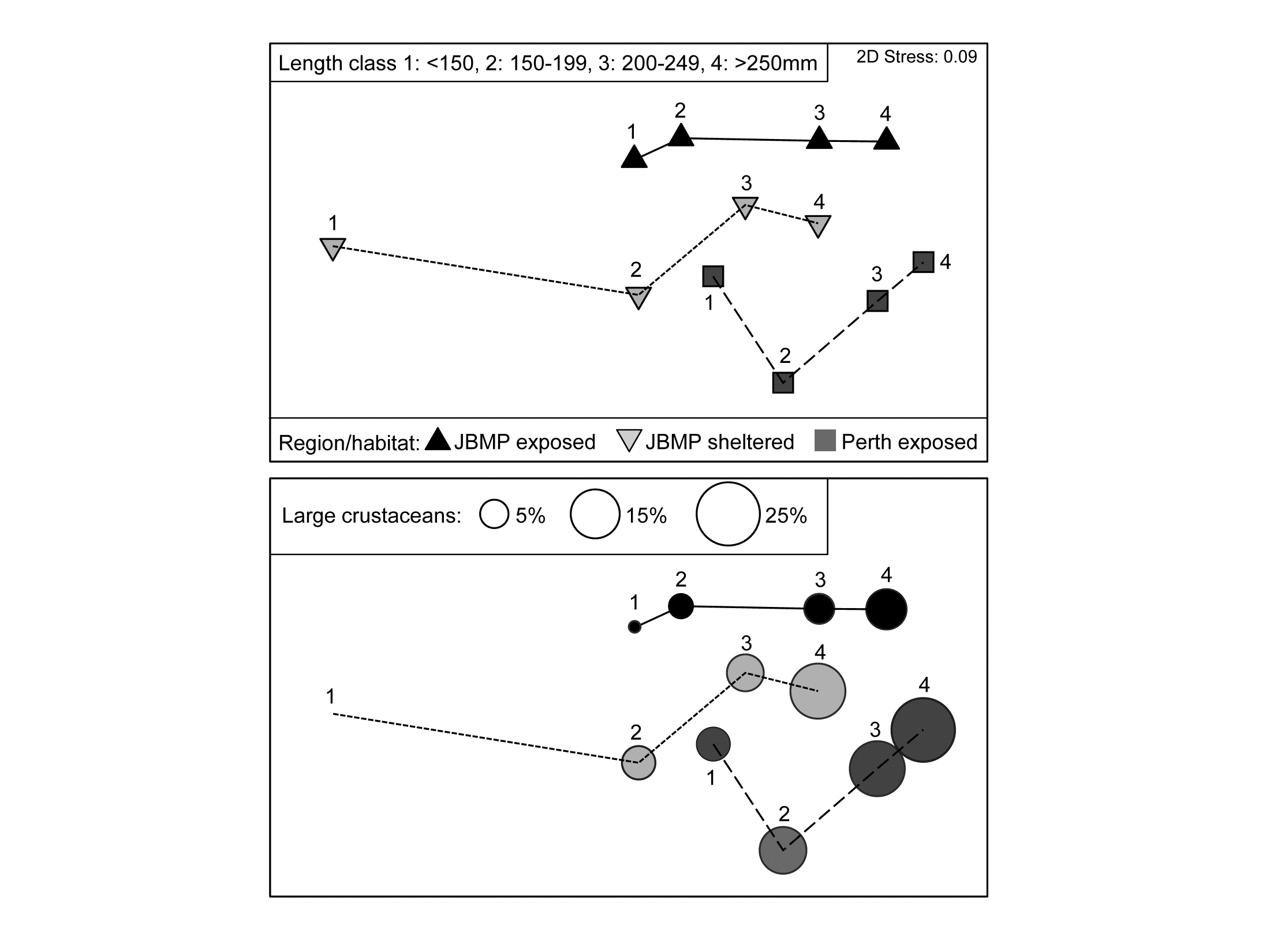 Fig. 6.15. King Wrasse diets {k}. nMDS (on Bray-Curtis) of $\sqrt{}$ taxon volumes averaged over replicates and seasonal periods, showing clear dietary change with King Wrasse body size and between regions/habitats; lower plot overlays bubbles with sizes proportional to one component of the average diet.
As for univariate ANOVA, the natural successor to hypothesis tests should be a means plot, illustrating these effect sizes. Since the period effect is absent, an average of the data matrix over both the 2 replicates and 2 periods is appropriate†. The resulting nMDS of the dietary assemblages for the 4 wrasse size-classes at the 3 locations is shown in Fig. 6.15. It has low stress (0.09) and displays the relationships seen in the tests with great clarity, unlike the high-stress (0.19) nMDS on the full set of samples, which is the typical ‘blob’ of replicate-level plots (an often useful mantra is: ‘test on the replicates – but ordinate the means’!).
The next question is always likely to be: ‘and which taxa are mainly implicated in the steady change in the dietary assemblage through the size classes?’. This is the subject of Chapter 7, but one of the simplest and most effective tools is a bubble plot, superimposing on each ordination point a circle (or in 3-d, a sphere) with size proportional to the (averaged) value for a specific taxon in that (averaged) sample. The lower plot in Fig. 6.15 shows a bubble plot for the ‘large crustaceans’, which are seen to become an increasing part of King Wrasse diet with size, in all locations.
¶ The original data potentially have a 5-factor crossed design, treating region and habitat separately and with 2 further common labrid species studied, but such higher-way designs can always be analysed at a lower level, flattening pairs of factors, as for A above. In fact, Lek, Fairclough, Platell et al. (2011) found it necessary to analyse only 3 factors at a time to explore dietary change with region, habitat, species, size and season because there were no sheltered sites on the Perth coast, and not all labrid species and not all size classes were found in each location. Examining different hypotheses may often require separate analysis of different selections from a data set, and you should not be reluctant to do this!
† Average the transformed data not the original matrix, or use the ‘distances among centroids’ option in PERMANOVA+, though again these give virtually identical plots, see footnote on page 5.9. The major step forward that PERMANOVA takes, albeit under the more restrictive assumptions of a linear model, is that it allows partitioning of the effects seen here into ‘main effects’ and ‘interactions’, something which is simply undefinable in a non-parametric approach (see later). Here, PERMANOVA tests give no evidence at all for any interactions: as the ordination shows, the orderly progression of diet as the wrasse grows is maintained in much the same way across the differing conditions (balance of food availability, in part, presumably) at the three locations.
6.16 Example: NZ kelp holdfast macrofauna
We now consider the fully nested design, C(B(A)). In north-eastern New Zealand, Anderson, Diebel, Blom et al. (2005) examined assemblages of invertebrates colonising kelp holdfasts at three spatial scales: 4 locations (A), with 2 sites (B) per location, sampling 2 areas (C) at each site and with 5 replicate holdfasts per area, {n}. This data is covered in detail in the PERMANOVA+ manual, Anderson, Gorley & Clarke (2008) ¶. Since B and C have only 2 levels, there can be no concept of them being ‘ordered’ or not; A is also seen as unordered. The test statistics are therefore $R$ and $\overline{R}$, case 3d in Table 6.4, giving for A: $R = 0.81$, B: $\overline{R}= 0.38$ and C: $\overline{R}= 0.26$.
These three ANOSIM R statistics are again directly comparable with each other. Their increase in size as the spatial scale increases is coincidental; they do not reflect accumulation of differences at all the spatial scales but only the additional assemblage differences when moving from replicates (with spacing at metres) to areas (at 10’s of metres) to sites (100’s of metres to kms) to locations (100’s of km). Thus, they can be seen as non-parametric equivalents of the univariate variance components (or the multivariate components of variation in PERMANOVA): the area differences
are small ($\overline{R} = 0.26$) in relation to assemblage variability from one holdfast to another, somewhat larger between sites (0.38), in relation to changes between areas, and very large among locations (0.81), relative to change in sites within those locations. This is in stark contrast to the conclusions one might draw from looking only at the significance levels (as seen from the permutation distributions under the null hypotheses, Fig. 6.16), A: p=1%, B: p=1.2%, C: p<<0.01%, a result of the very different numbers of replicates, and thus possible permutations (105, 85 and 1268). As always, it is the $R$ values which give the effect sizes.
Fig. 6.16. NZ kelp holdfast fauna {n}. Null distributions by permutation for 3-factor fully nested (unordered) ANOSIM tests, C(B(A)), with 5 replicates from each of 2 areas (C), nested in 2 sites (B), nested in 4 locations (A). Very large numbers of permutations possible for the lowest level test of areas, so 9999 selected at random; all permutations are computed for site test (81) and location test (105).
Pairwise tests are only meaningful at the top level of such a nested design and there are insufficient permutations here (3) to make these at all informative. The best way, as always, to follow up the global ANOSIM tests, and visualise the effect sizes, is an MDS based on averaged data (but see footnotes on pages 5.9 & 6.15). Here Fig. 6.17 averages the (square root-transformed) replicate counts for the 16 areas, recomputes Bray-Curtis and the nMDS plot re-affirms the test results.
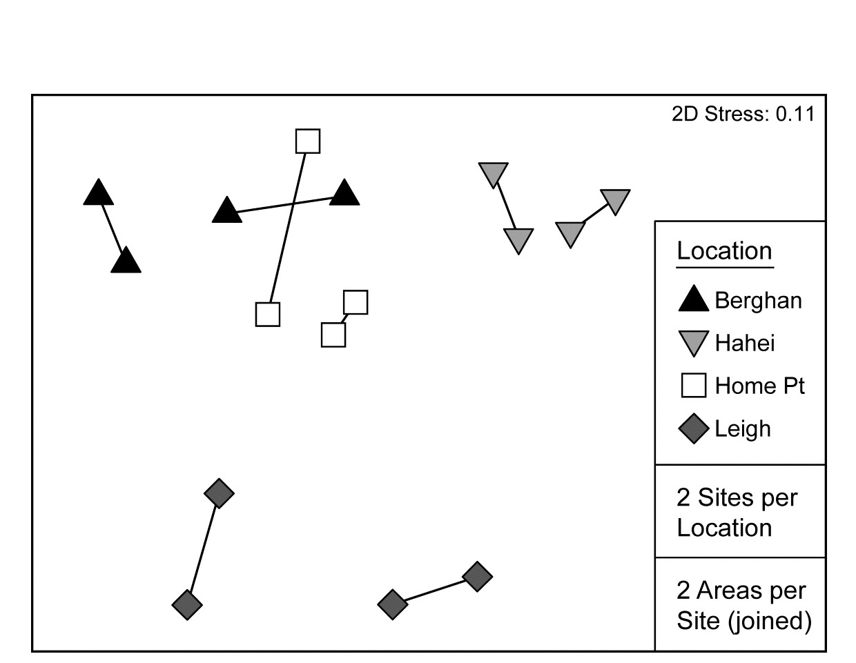
Fig. 6.17. NZ kelp holdfast fauna {n}. nMDS (on Bray-Curtis) of square-rooted abundances of 351 species, averaged over five replicates holdfasts in each area (nested in site and location).
There is a minor technical issue, in the sequence of nested ANOSIM tests, as to how best to combine the original replicates to provide ‘area replicates’ for a test of site, and then how best to combine the areas to provide ‘site replicates’ for a test of locations. There are many possibilities: PERMANOVA uses centroids calculated in the high-dimensional resemblance space (see Anderson, Gorley & Clarke (2008) ) whereas the rank-based approach in PRIMER was given on page 6.6 for the two-way nested case (the original resemblances are ranked, then averaged and re-ranked, at each level). Averaging the similarities rather than their ranks is another possibility, as is averaging the data, both transformed (as in Fig. 6.17) or untransformed. Only slight variations would be likely from the different choices, though experience suggests that averaging untransformed data makes the greatest difference. But in one situation even this might be considered appropriate, namely when the original replicates are sufficiently sparse and unreliable not to constitute a fair reflection of the assemblage structure at all: to pool them (i.e. average untransformed counts) and run the 3-way nested case as 2-way nested for A and B(A) tests (2g-n, Table 6.3) might then be preferable.
¶ We are ignoring for the purposes of this illustration that, as Anderson, Gorley & Clarke (2008) explain, the holdfasts will have different volumes and, even after we have attempted to correct for this by standardising all samples to relative composition not absolute numbers, there may still be some artefactual dissimilarity arising from higher species richness in larger holdfasts. PERMANOVA tests can attempt to model the ‘nuisance’ effects of covariates such as this, through a linear regression, and thereby adjust the C(B(A)) tests (as Anderson, Gorley & Clarke (2008) do in this case); clearly nothing similar could ever be available in the non model-based approach here. However, such biases from unequal sample sizes will still remain in any ordination configuration, whatever the approach, and it should be examined by bubble plots of (here) holdfast volume on the area MDS. Characteristic indicators of a problem are that all the outlying points have low sample volumes (which does not happen here). Presence/absence analyses will be most prone to this artefact, so where such a problem is expected, some amelioration is likely from using less severe transforms – here the mild square root is used – or possibly dispersion weighting (Chapter 9). This downweights the contribution of highly abundant, but highly variable, species without also effectively ‘squashing’ species with low counts (but consistent over replicates) to presence/absence, as severe transformations will do.
6.17 Example: Tees Bay macrofauna
The final example in this chapter is of a mixed nested and crossed design B$\times$C(A), for a total of 192 macrobenthic samples (282 species) from: A: four sub-tidal Areas of Tees Bay (Fig. 6.18, top left), with C: two Sites from each area, the same sites being returned to each September over B: 24 Years (1973-1996), part of a wider study of the Tees estuary, Warwick, Ashman, Brown et al. (2002) , {t}. Sites (C) are therefore nested in Areas (A) but crossed with Years (B). There was a further level of replication, with multiple grab samples collected but these have been averaged to give a more reliable picture of the assemblage on that occasion (the repeat grabs from a single ship stationing being considered ‘pseudo-replicates’ in time, and possibly space). The areas lie on a spatial transect (c. 5km spacing) but are probably not ordered hydrodynamically, so we shall contrast both ordered and unordered tests for A (cases 3m/3j in Table 6.4). The years are also amenable to analysis under either assumption: as it happens, there is a clear annual trend in assemblage structure over the period (seen in the right-hand plots of Fig. 6.18, for the two sites in each area averaged), but the prior expectation might have been for a more complex time signal of cycles or short-term changes and reversions, so this data will serve as an illustration of both the case of B ordered or unordered (cases 3l/3j). There being only two sites in each area, it is then irrelevant whether C is considered ordered or not; with no real replication, there can be no test for a site effect from only two sites (though there would be a test with a greater number of sites, either ordered or not, 3k/3j).
Fig. 6.18. Tees Bay macrofauna {t}. Map of four sampling areas in Tees Bay, NE England, and separate nMDS time-series plots for each area, of the macrobenthic assemblages over 24 years of September sampling; abundances were fourth-root transformed then averaged over the two sites in each area, then input to Bray-Curtis similarity calculation. Bottom left plot is the nMDS of averages of transformed abundances over the 24 time points for the two sites (a-b, c-d, e-f, g-h) in each of the four areas.
Test for Area factor (A)
The schematic below displays the construction of the ANOSIM permutation test for area (A), case 3m/3j¶.

The building blocks are the 1-way ANOSIM statistics $R$ (or $R^{Oc}$ if A is considered ordered) for a test of the 4 areas, using as replicates the 2 sites in each area, computed separately for each year. These are then averaged over the 24 years, to obtain the overall test statistic for A of $\overline{R}$ (or $\overline{R}^{Oc}$), exactly as for the usual 2-way crossed case A$\times$B met on page 6.7. The crucial difference however is in generating the null hypothesis distribution for this test statistic. Permuting the 8 sites across the 4 areas separately for each year, as the standard A$\times$B test would do, is to assume that the sites are randomly drawn afresh each year from the defined area, rather than determined only once and then revisited each year. The relevant permutation is therefore to keep the columns of this schematic table intact and shuffle the 8 whole columns randomly over the 4 areas, recalculating $\overline{R}$ (or $\overline{R}^{Oc}$) each time. There will be many fewer permutations for the A test under this B$\times$C(A) design (8!/2!2!2!2!4! =105 for the unordered case, compared with $105^{24}$) but what it loses in ‘power’ here it may make up for in improved focus when examining the time factor: subtle assemblage changes from year to year may be seen by returning to the same site(s), and these might otherwise get swamped by large spatial variability from site to site, if the latter are randomly reselected each year.
If area is considered an unordered factor, $\overline{R}= 0.60$, a high value (and the most extreme of the 105 permutations, so p = 1%); this is clearly seen in the time-averaged MDS plot for the 8 sites (Fig. 6.18, lower left). If treated as an ordered factor, the area test gives $\overline{R}^{Oc} = 0.13$, now not even significant. These two $\overline{R}$ values are directly comparable; both are slopes of a linear regression of the type seen in Fig. 6.13b, with the same y axis values but only two rather than four x axis points in the unordered case (within and among groups, as earlier explained). The MDS plot of sites in Fig. 6.18 makes clear the down side of an ordered test, based solely on the NW to SE transect of areas: here the middle two areas are within the confines of Tees Bay, their assemblages potentially influenced by the hydrodynamics or even anthropogenic discharges from the Tees estuary. Thus areas 1 and 4 are rather similar to each other but differ from areas 2 and 3. Opting for what can be a more powerful test if there is a serial pattern risks failing to detect obvious differences when they are not serial, as illustrated below for one of the 24 components of the average $\overline{R}$ and $\overline{R}^{Oc}$, namely the $R$ and $R^{Oc}$ constructions for 1978:
Test for Year factor (B)
Turning to the test for the Year factor (B), case 3l/3j in Table 6.4, the schema for construction of the test statistic in both ordered and unordered cases is now:
When years are considered ordered, the test reduces to the 2-way crossed layout B$\times$C (case 2d, Table 6.3) in which a 1-way ordered ANOSIM statistic without replicates ($R^{Os}$) is calculated over years, separately for each of the 8 sites, and these values averaged to give $\overline{R}^{Os}$, exactly the test for trend seen in Fig. 6.14 for the Phuket coral reef data (though there the trend was for spatial positions averaged over years, whilst here it is the opposite, of inter-annual trends averaged over sites). The appropriate permutation is the usual one of samples in each site being randomly permuted across the years (since the null hypothesis specifies that there is no year effect, at any site). As Fig. 6.18 illustrates, this will be roundly rejected, with global $\overline{R}^{Os} = 0.52$, which is significant at any fixed level, in effect, as shown by the null permutation distribution:

If it is considered unwise to test only for a time trend, rather than a more general pattern of annual changes, there is no replication which the test for B can exploit so the design falls back on an indirect test of the type introduced in Fig. 6.9: evidence of differences among years is provided by a commonality of time patterns in space. A modified test statistic is needed here to cope with the structuring of the spatial factors into a 2-way nested design of sites within areas. As shown in the above schematic diagram, a logical construction for the test statistic here is to use the matching statistic $\rho_{av}$ among the sites within each area (though in this case there is only one $\rho$ since there are only 2 sites) and then average this across the areas, to give a doubly-averaged $\overline{\rho}_ {av}$ statistic. If there are no annual differences this will, as usual, take the value zero, and the null hypothesis distribution is created by the same permutations as for the ordered test. An inter-annual effect is therefore inferred from consistency in time patterns between sites. If (as might well be thought in this context) it is more appropriate to infer consistent temporal change by noting commonality at the wider spatial scale of areas, then the sites should simply be averaged (see previous footnotes on how best to do this) to leave a 2-way A$\times$B design with both factors unordered, and the B test uses the (singly-averaged) $\rho_{av}$ statistic of Fig. 6.9.
Generally one might expect the time pattern to be less consistent as the spatial scale widens, but here, based on sites, $ \overline{\rho}_ {av} = 0.62$ and on areas, $\rho_ {av} = 0.66$, perhaps because averaging sites removes some of the variability in the sampling. Both $\rho$ statistics are again highly significant, though note that they cannot be compared with the $\overline{R}^{Os}$ value for the ordered case; the statistics are constructed differently.
Returning to the $\overline{R}^{Os}$ test for temporal trend, doubly averaging the statistics in that case, by site then area, could not actually change the previous value (0.52), though averaging sites first and performing the 2-way design on areas $\times$ years does increase the value to $\overline{R}^{Os} = 0.60$, for the same reasons of reduction in sampling ‘noise’; it is this statistic that reflects the overall trend seen in the four right-hand plots of Fig. 6.18. It would generally be of interest to ask whether the averaged $\overline{R}^{Os}$ hides a rather different trend for each area, and the individual trend values $R^{Os}$ for each area (or site) could certainly be calculated and tested. The 4 areas here give the reasonably consistent values $R^{Os}$ = 0.67, 0.54, 0.50, 0.67 respectively (all p<<0.01%), though there is perhaps a suggestion here and in the plots that the wider regional trend seen in Areas 1 and 4, and for which there is evidence from other North Sea locations (a potential result of changing hydrodynamics), is being impacted by more local changes within the Tees estuary, which will affect areas 2 and 3, within Tees Bay. This is a form of interaction between Year and Area factors and we shall see later that limited progress can be made in exploring this type of interaction non-parametrically, through the definition of second-stage MDS and tests (Chapter 16). These ask the question “does the assemblage temporal pattern change between areas, in contrast with its fluctuation within an area?”, and the comparison becomes one between entire time sequences rather than between individual multivariate samples.
This raises the following important issue about the limitations of non-parametric tests in exploring the conventional interactions of additive linear models.
Partitioning
One crucial point needs to be made about all the 2- and 3-way tests of this chapter. They are fully non-parametric, being based only on the rank order of dissimilarities, which delivers great robustness, but they cannot deliver the variance partitioning found in the semi-parametric methods of PERMANOVA+, the add-on routines to PRIMER ( Anderson, Gorley & Clarke (2008) ). PERMANOVA uses the precise measurement scale of the dissimilarities to fit general linear models in the high-dimensional PCO ‘resemblance space’ and it is then able to partition effects of a factor into main effects and 2-way (or 3-way or higher) interactions, each of which can then be tested. For some scientific questions, testing for the presence or absence of an interaction is the only form of inference that will suffice: a good example would be for Before-After/ Control-Impact (BACI) study designs, and there are many further examples in Anderson, Gorley & Clarke (2008) and associated papers. The non-parametric ANOSIM routine cannot (and could never) do this linear model variance-partitioning, of effects into main effects and interactions, because this form of interaction is a purely metric concept. This is simply illustrated in the univariate case by a hypothetical 2-factor crossed design with two levels for both A and B (e.g. where the response variable y is clearance rate of particles by a filter-feeding species under A1: low density and A2: high density of particulates, and B1: at night, B2: during the day), let us suppose with minimal variance in the replicates, giving cell means of (left-hand side):
The data matrix for variable y demonstrates that there is significant interaction between particle density and day/night factors, because the means are not additive: the difference in clearance rate between high and low density is not the same during the night (1) as during the day (4). But a simple log$_2$ transform of y gives the table to the right, in which there is now no interaction between the factors: the difference between logged clearance rate at low and high particle density is the same during both day and night (1). Yet, both these tables are identical if viewed non-parametrically, i.e. with the values replaced by their ranks.
This example is scarcely representative of the typical multivariate abundance matrix but it does illustrate that this simple form of interaction is essentially a parametric construction, based on linear models of adding main effects, interactions and error. Though, as previously mentioned, ‘non-parametric interaction’ is not an altogether invalid concept (see Chapter 16), it cannot be straightforwardly defined. The ANOSIM crossed designs are tests for the presence or otherwise of an effect of factor A; this may be a large effect at one level of another factor B, and smaller ones at its other levels, or it may be a more consistent effect of A at all levels of B – these situations are not distinguished, and one way of viewing these $\overline{R}$ statistics is as combinations of ‘main effects’ and ‘interactions’. What they tell you, robustly, is whether factor A has an overall effect, at least somewhere, having removed all contributions that the other crossed factor(s) could possibly be having. They do not do this by subtracting some estimate under a general linear model of the effect of other terms. Their excision of other factors is more surgical than that: they only ever compare the different levels of A under an identical level for all other combinations of factors. Therefore there can be no equivalent, for example, of the way that in linear models main effects can apparently disappear because interactions ‘in different directions’ cancel them out. An $\overline{R}$ statistic is perfectly meaningful in the presence of interactions. Under the null hypothesis, the component R values making up that average are all approximately zero; where there are effects some or all of those R values become positive. If enough of them do so (or one or two of them do so enough), an effect is detected.
¶ It is to be understood that each dot represents a sample of 282 species abundances (going into the page, if you like). Of course, data is not input into PRIMER in this (3-way) format but in the usual species $\times$ (all) samples worksheet, with areas (1-4), years (73-96) and sites (a-h) identified in the associated factors sheet.
6.18 Recommendations
-
For typical species abundance matrices, it is much preferable to use a non-parametric ANOSIM-type permutation test rather than classical MANOVA; the latter will almost always be totally invalid. A realistic alternative is the semi-parametric PERMANOVA tests of Anderson, Gorley & Clarke (2008) . These do make more assumptions, fitting additive linear models in a (complex) high-dimensional space defined by the (metric) resemblance matrix but, crucially, do not make unacceptable normality assumptions in carrying out their tests, which use (approximate) null distributions from permutation procedures. In simple designs, ANOSIM’s greater robustness might be preferred; in more complex designs some questions can only be answered by PERMANOVA. This is a familiar balance from univariate statistics: non-parametric methods are more robust but give shallower inference, model estimation of parameters inevitably involves more assumptions but allows a deeper level of inference.
-
Choice of the level and type of replication should be carefully considered. Though it is difficult to define power for any of the ANOSIM (or PERMANOVA) tests, it is important to ensure sufficient samples are taken at the right level to generate enough permutations for meaningful significance levels. Equally important is that replicates which are crucial for the tests being undertaken should genuinely represent the condition being sampled: pseudo-replication is commonplace, e.g. analyses of sub-cores of single cores, or sets of spatially contiguous or temporally coincident samples which are unrepresentative of the extent of the sites or times about which inference is desired. Pseudo-replicates may still have an important role, when pooled, in providing enough material for sensible definition of a single replicate of that time or place, but the balance of collection or analysis effort at different levels of a design is often context dependent, and pilot experimentation will usually reap dividends for efficiency of the main study. As a general rule, design to provide fully representative replication at the level immediately below the effect of main interest, and use balanced crossed designs to eliminate non-negligible factors which are not the main focus of the study.
-
A point that cannot be over-stressed is that ANOSIM tests only apply to groups of samples specified prior to seeing (or collecting) the data. A dangerous misconception is that one can use a cluster analysis of the species abundance data to define sample groupings whose statistical validity can be established by performing an ANOSIM test for differences among those groups. This is entirely wrong, the reasoning being completely circular. Sometimes, independent data exists (e.g. environmental) which can permit the definition of groups to test with the biotic data. Another safe course here can be to use a first set of (biotic) data to define the groups of interest, i.e. to erect the hypothesis, and then to collect a further set of the same assemblage data to test that hypothesis. Alternatively, the SIMPROF procedure of Chapter 3 may allow you to make some (weaker) statements about structure in the data that is worth exploring in future studies. If prior structure exists, use it: where ANOSIM (or PERMANOVA) tests are valid, they are your most useful testing tools.