Chapter 9: Transformations and dispersion weighting
- 9.1 Introduction
- 9.2 Univariate case
- 9.3 Multivariate case
- 9.4 Recommendations
- 9.5 Dispersion weighting
- 9.6 Example: Fal estuary copepods
- 9.7 Variability weighting
9.1 Introduction
There are two distinct roles for transformations in community analyses:
a) to validate statistical assumptions for parametric techniques – in the approach of this manual such methods are restricted to univariate tests;
b) to weight the contributions of common and rare species in the (non-parametric) multivariate representations.
The second reason is the only one of relevance to the preceding chapters, with the exception of Chapter 8 where it was seen that standard parametric analysis of variance (ANOVA) could be applied to diversity indices computed from replicate samples at different sites or times. Being composite indices, derived from all species counts in a sample, some of these will already be approximately continuous variates with symmetric distributions, and others can be readily transformed to the normality and constant variance requirements of standard ANOVA. Also, there may be interest in the abundance patterns of individual species, specified a priori (e.g. keystone species), which are sufficiently common across most sites for there to be some possibility of valid parametric analysis after transformation.
9.2 Univariate case
For purely illustrative purposes, Table 9.1 extracts the counts of a single Thyasira species from the Frierfjord macrofauna data {F}, consisting of four replicates at each of six sites.
Table 9.1. Frierfjord macrofauna {F}. Abundance of a single species (Thyasira sp.) in four replicate grabs at each of the six sites (A–E, G).
| Site: | A | B | C | D | E | G |
|---|---|---|---|---|---|---|
| Replicate | ||||||
| 1 | 1 | 7 | 0 | 1 | 62 | 66 |
| 2 | 4 | 0 | 0 | 8 | 102 | 68 |
| 3 | 3 | 3 | 0 | 5 | 93 | 52 |
| 4 | 11 | 2 | 3 | 13 | 69 | 36 |
| Mean | 4.8 | 3.0 | 0.8 | 6.8 | 81.8 | 55.5 |
| Stand. dev. | 4.3 | 2.9 | 1.5 | 5.1 | 18.7 | 14.8 |
Two features are apparent:
-
the replicates are not symmetrically distributed (they tend to be right-skewed);
-
the replication variance tends to increase with increasing mean, as is clear from the mean and standard deviation (s.d.) values given in Table 9.1.
The lack of symmetry (and thus approximate normality) of the replication distribution is probably of less importance than the large difference in variability; ANOVA relies on an assumption of constant variance across the groups. Fortunately, both defects can be overcome by a simple transformation of the raw data; a power transformation (such as a square root), or a logarithmic transformation, have the effect both of reducing right-skewness and stabilising the variance.
Power transformations
The power transformations $y ^ * = y ^ \lambda$ form a simple and useful family, in which decreasing values of $\lambda$ produce increasingly severe transformations. The log transform, $y ^ * =\log _ e (y)$, can also be encompassed in this series (technically, $(y ^ \lambda-1)/\lambda \rightarrow \log _ e (y)$ as $\lambda \rightarrow 0$). Box & Cox (1964) give a maximum likelihood procedure for optimal selection of $\lambda$ but, in practice, a precise value is not important, and indeed rather artificial if one were to use slightly different values of $\lambda$ for each new analysis. The aim should be to select a transformation of the right order for all data of a particular type, choosing only from, say: none, square root, 4th root or logarithmic. It is not necessary for a valid ANOVA that the variance be precisely stabilised or the non-normality totally removed, just that gross departures from the parametric assumptions (e.g. the order of magnitude change in s.d. in Table 9.1) are avoided. One useful technique is to plot log(s.d.) against log(mean) and estimate the approximate slope of this relationship ($\beta$). This is shown here for the data of Table 9.1.

It can be shown that, approximately, if $\lambda$ is set roughly equal to $1 – \beta$, the transformed data will have constant variance. That is, a slope of zero implies no transformation, 0.5 implies the square root, 0.75 the 4th root and 1 the log transform. Here, the square root is indicated and Table 9.2 gives the mean and standard deviations of the root-transformed abundances: the s.d. is now remarkably constant in spite of the order of magnitude difference in mean values across sites. An ANOVA would now be a valid and effective testing procedure for the hypothesis of ‘no site-to-site differences’, and the means and 95% confidence intervals for each site can be back-transformed to the original measurement scales for a more visually helpful plot.
Table 9.2. Frierfjord macrofauna {F}. Mean and standard deviation over the four replicates at each site, for root-transformed abundances of Thyasira sp.
| Site: | A | B | C | D | E | G |
|---|---|---|---|---|---|---|
| Mean(y*) | 2.01 | 1.45 | 0.43 | 2.42 | 9.00 | 7.40 |
| S.d.(y*) | 0.97 | 1.10 | 0.87 | 1.10 | 1.04 | 1.04 |
Like all illustrations, though genuine enough, this one works out too well to be typical! In practice, there is usually a good deal of scatter in the log s.d. versus log mean plots; more importantly, most species will have many more zero entries than in this example and it is impossible to ‘transform these away’: species abundance data are simply not normally distributed and can only rarely be made so. Another important point to note here is that it is never valid to ‘snoop’ in a data matrix of, perhaps, several hundred species for one or two species that display apparent differences between sites (or times), and then test the significance of these groups for that species. This is the problem of multiple comparisons referred to in Chapter 6; a purely random abundance matrix will contain some species which fallaciously appear to show differences between groups in a standard 5% significance level ANOVA (even were the ANOVA assumptions to be valid). The best that such snooping can do, in hypothesis testing terms, is identify one or two potential key or indicator species that can be tested with an entirely independent set of samples.
These two difficulties between them motivate the only satisfactory approach to most community data sets: a properly multivariate one in which all species are considered in combination in non-parametric methods of display and testing, which make no distributional assumptions at all about the individual counts.
9.3 Multivariate case
There being no necessity to transform to attain distributional properties, transformations play an entirely separate (but equally important) role in the clustering and ordination methods of the previous chapters, that of defining the balance between contributions from common and rarer species in the measure of similarity of two samples.
Returning to the simple example of Chapter 2, a subset of the Loch Linnhe macrofauna data, Table 9.3 shows the effect of a 4th root transformation of these abundances on the Bray-Curtis similarities. The rank order of the similarity values is certainly changed from the untransformed case, and one way of demonstrating how dominated the latter is by the single most numerous species (Capitella capitata) is shown in Table 9.4. Leaving out each of the species in turn, the Bray-Curtis similarity between samples 2 and 4 fluctuates wildly when Capitella is omitted in the untransformed case, though changes much less dramatically under 4th root transformation, which downweights the effect of single species.
Table 9.3. Loch Linnhe macrofauna {L} subset. Untransformed and 4th root-transformed abundances for some selected species and samples (years), and the resulting Bray-Curtis similarities between samples.
| Untransformed | ||||||||||
|---|---|---|---|---|---|---|---|---|---|---|
| Sample: | 1 | 2 | 3 | 4 | ||||||
| Species | Sample | 1 | 2 | 3 | 4 | |||||
| Echinoca. | 9 | 0 | 0 | 0 | 1 |
– | ||||
| Myrioche. | 19 | 0 | 0 | 3 | 2 |
8 | – | |||
| Labidopl. | 9 | 37 | 0 | 10 | 3 |
0 | 42 | – | ||
| Amaeana | 0 | 12 | 144 | 9 | 4 |
39 | 21 | 4 | – | |
| Capitella | 0 | 128 | 344 | 2 | ||||||
| Mytilus | 0 | 0 | 0 | 0 | ||||||
| $\sqrt{} \sqrt{}$-transformed | ||||||||||
| Sample: | 1 | 2 | 3 | 4 | ||||||
| Species | Sample | 1 | 2 | 3 | 4 | |||||
| Echinoca. | 1.7 | 0 | 0 | 0 | 1 |
– | ||||
| Myrioche. | 2.1 | 0 | 0 | 1.3 | 2 |
26 | – | |||
| Labidopl. | 1.7 | 2.5 | 0 | 1.8 | 3 |
0 | 68 | – | ||
| Amaeana | 0 | 1.9 | 3.5 | 1.7 | 4 |
52 | 68 | 42 | – | |
| Capitella | 0 | 3.4 | 4.3 | 1.2 | ||||||
| Mytilus | 0 | 0 | 0 | 0 |
Transformation sequence
The previous remarks about the family of power transformations apply equally here: they provide a continuum of effect from $\lambda = 1$ (no transform), for which only the common species contribute to the similarity, through $\lambda = 0.5$ (square root), which allows the intermediate abundance species to play a part, to $\lambda = 0.25$ (4th root), which takes some account also of rarer species. As noted earlier, $\lambda \rightarrow 0$ can be thought of as equivalent to the $\log _ e (y)$ transformation and the latter would therefore be more severe than the 4th root transform. However, in this form, the transformation is impractical because the (many) zero values produce $\log(0) \rightarrow - \infty$. Thus, common practice is to use $\log(1+y)$ rather than $\log(y)$, since $\log(1+y)$ is always positive for positive $y$ and $\log(1+y)= 0$ for $y = 0$. The modified transformation no longer falls strictly within the power sequence; on large abundances it does produce a more severe transformation than the 4th root but for small abundances it is less severe than the 4th root. In fact, there are rarely any practical differences between cluster and ordination results performed following $y ^ {0.25}$ or $\log(1+y)$ transformations; they are effectively equivalent in focusing attention on patterns within the whole community, mixing contributions from both common and rare species.¶
Table 9.4. Loch Linnhe macrofauna {L} subset. The changing similarity between samples 2 and 4 (of Table 9.3) as each of the six species is omitted in turn, for both untransformed and 4th root-transformed abundances.
| Species omitted: | None | 1 | 2 | 3 | 4 | 5 | 6 |
| Bray-Curtis (S): | 21 | 21 | 21 | 14 | 13 | 54 | 21 |
| $\sqrt{} \sqrt{}$-transformed | |||||||
| Species omitted: | None | 1 | 2 | 3 | 4 | 5 | 6 |
| Bray-Curtis (S): | 68 | 68 | 75 | 61 | 59 | 76 | 68 |
The logical end-point of this transformation sequence is therefore not the log transform but a reduction of the quantitative data to presence/absence, the Bray-Curtis coefficient (say) being computed on the resulting matrix of 1’s (presence) and 0’s (absence). This computation is illustrated in Table 9.5 for the subset of the Loch Linnhe macrofauna data used earlier. Comparing with Table 9.3, note that the rank order of similarities again differs, though it is closer to that for the 4th root transformation than for the untransformed data. In fact, reduction to presence/absence can be thought of as the ultimate transformation in down-weighting the effects of common species. Species which are sufficiently ubiquitous to appear in all samples (i.e. producing a 1 in all columns) clearly cannot discriminate between the samples in any way, and therefore do not contribute to the final multivariate description. The emphasis is therefore shifted firmly towards patterns in the intermediate and rarer species, the generally larger numbers of these tending to over-ride the contributions from the few numerical or biomass dominants.
Table 9.5. Loch Linnhe macrofauna {L} subset. Presence (1) or absence (0) of the six species in the four samples of Table 9.3, and the resulting Bray-Curtis similarities.
| Presence/absence | |||||||||
|---|---|---|---|---|---|---|---|---|---|
| Sample: | 1 | 2 | 3 | 4 | |||||
| Species | Sample | 1 | 2 | 3 | 4 | ||||
| Echinoca. | 1 | 0 | 0 | 0 | 1 |
– | |||
| Myrioche. | 1 | 0 | 0 | 1 | 2 |
33 | – | ||
| Labidopl. | 1 | 1 | 0 | 1 | 3 |
0 | 80 | – | |
| Amaeana | 0 | 1 | 1 | 1 | 4 |
57 | 86 | 67 | – |
| Capitella | 0 | 1 | 1 | 1 | |||||
| Mytilus | 0 | 0 | 0 | 0 |
One inevitable consequence of ‘widening the franchise’ in this way, allowing many more species to have a say in determining the overall community pattern, is that it will become increasingly harder to obtain 2-d ordinations with low stress: the view we have chosen to take of the community is inherently high-dimensional. This can be seen in Fig. 9.1, for the dosing experiment {D} in the Solbergstrand mesocosm (GEEP Oslo workshop), previously met in Figs. 4.2 and 5.6. Four levels of contaminant dosing (designated Control, Low, Medium, High) were each represented by four replicate samples of the resulting nematode communities, giving the MDS ordinations of Fig. 9.1. Note that as the severity of the transformation increases, through none, root, 4th root and presence/absence (Fig. 9.1a to 9.1d respectively), the stress values rise from 0.08 to 0.19.

Fig 9.1 Dosing experiment, Solbergstrand {D}. MDS of nematode communities in four replicates from each of four treatments (C = control, L = low, M = medium, H = high dose of a hydrocarbon/copper contaminant mixture dosed to mesocosm basins), based on Bray-Curtis similarities from transformed data: a) no transform (stress = 0.08), b) $\sqrt{}$ (stress = 0.14), c) $\sqrt{} \sqrt{}$ (stress = 0.18), d) presence/absence (stress = 0.19).
It is important to realise that this is not an argument for deciding against transformation of the data. Fig. 9.1a is not a better representation of the between-sample relationships than the other plots: it is a different one. The choice of transformation is determined by which aspects of the community we wish to study. If interest is in the response of the whole community then we have to accept that it may be more difficult to capture this in a low-dimensional picture (a 3-d or higher-dimensional MDS may be desirable). On the other hand, if the data are totally dominated by one or two species, and it is these that are of key biological interest, then of course it will be possible to visualise in a 1- or 2-d picture how their numbers (or biomass) vary between samples: in that case an ordination on untransformed data will be little different from a simple scatter plot of the counts for the two main species.
¶ Though practical differences are likely to be negligible, on purely theoretical grounds it could be argued that the 4th root is the more satisfactory of the two transformations because Bray-Curtis similarity is then invariant to a scale change in y. Similarity values would be altered under a log(1+y) transformation if abundances were converted from absolute values to numbers per $m^2$ of the sampled substrate, or if biomass readings were converted from mg to g. This does not happen with a strict power transformation; it is clear from equation (2.1) that any multiplying constant applied to y will cancel on the top and bottom lines of the summations.
9.4 Recommendations
The transformation sequence in a multivariate analysis, corresponding to a progressive downweighting of the common species, is effectively:
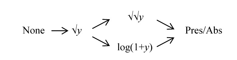
The choice of transformation from this sequence can affect the conclusions of an analysis, and in many respects it is more a biological than a statistical question: which view of the community do we wish to take (shallow or deep), given that there are potentially many different 2-dimensional summaries of this high-dimensional data?
Statistical considerations do enter, however, particularly in relation to the reliability of sampling. At one extreme, a presence/absence analysis can give too much weight to the chance capture of species only found occasionally as single individuals. At the other extreme, an abundance MDS plot can be distorted by the capture of larvae or opportunist colonisers with a strong degree of spatial clumping, such that replicate samples at the same time/location give counts from absent to thousands. Under certain conditions, e.g. when the data matrix consists of real counts (not adjusted densities per area of sediment or volume of water) and there are replicate samples which will allow the degree of clumping of individuals to be quantified, the next section describes a useful way of removing the effects of this clumping (by dispersion weighting). This replaces the statistical need for transformation (to reduce highly erratic counts over replicates) but not necessarily the biological need, which remains that of balancing contributions from (consistently) abundant with less abundant species.
If conditions do not allow dispersion weighting (e.g. absence of replicates), the practical choice of transformation is often between moderate ($\sqrt{}$) and rather severe ($\sqrt{} \sqrt{}$ or log), retaining the quantitative information but downplaying the species dominants. (After dispersion weighting the severest transformations are not usually necessary). Note that the severe transformations come close to reducing the original data to about a 6 point scale: 0 = absent, 1 = one individual, 2 = handful, 3 = sizeable number, 4 = abundant, ≥5 = very abundant. Rounding the transformed counts to this discrete scale will usually make little or no difference to the multivariate ordination (though this would not be the case for some of the univariate and graphical methods of Chapter 8). The scale may appear crude but is not unrealistic; species densities are often highly variable over small-scale spatial replication, and if the main requirement is a multivariate description, effort expended in deriving precise counts from a single sample could be better spent in analysing more samples, to a less exacting level of detail. This is also a central theme of Chapter 10.
9.5 Dispersion weighting
There is a clear dichotomy, in defining sample similarities, between methods which give each variable (species) equal weight, such as normalisation or species standardisation, and those which treat counts (of whatever species) as comparable and therefore give greater weight to more numerically dominant species. As pointed out above, giving rare species the same weight as dominant ones bundles in a great deal of ‘noise’, diffusing the ‘signal’, but it can be equally unhelpful to allow the analysis to be driven by highly abundant, but very erratic counts, from motile species occurring in schools, or more static species which are spatially clumped by virtue of their colonising or reproductive patterns. A severe transformation will certainly reduce the dominance of such species, but it can be seen as rather a blunt instrument, since it also squeezes out much of the quantitative information from mid- or low-abundance species, some of which may not exhibit this erratic behaviour over replicates of the same condition (site/time/treatment), because they are not spatially clumped. If data are genuinely counts and information from replicates is available, a better solution ( Clarke, Chapman, Somerfield et al. (2006) ) is to weight species differently, according to the reliability of the information they contain, namely the extent to which their counts in replicates display overdispersion.
It is important to appreciate the subtlety of the idea of dispersion weighting: species are not down-weighted because they show large variation across the full set of samples; they may do that because their abundance changes strongly across the different conditions (and it is precisely those species which will best indicate community change). Species are down-weighted if they have high variability, for their mean count, in replicates of the same condition. In fact, we must be careful to make no use of information about the way abundances vary across conditions when determining the weight each species gets in the analysis, otherwise we are in serious danger of a self-fulfilling argument (e.g. high weight given to species which, on visual inspection, appear to show the greatest differences between groups will clearly bias tests unfairly in favour of demonstrating community change, just as surely as picking out only a subset of species, a posteriori, to input to the analyses).
Dispersion weighting (DW) therefore simply divides all counts for a single species by a particular constant, calculated as the index of dispersion D (the ratio of the variance to the mean) within each group, averaged across all groups to give divisor $\overline{D}$ for that species. The justification for this is a rather simple but general model in which counts of a species in each replicate are from a generalised Poisson distribution. Details are given in Clarke, Chapman, Somerfield et al. (2006) , but the concept is illustrated in Fig. 9.2, thought of as replicate quadrats ‘catching’ a different number of centres of population (clumps) for that species as the conditions (groups) change, but with each centre containing a variable number of individuals, with unknown probability distribution. The only assumption is that the different conditions change the number of clumps but not the average or standard deviation of the clump size, e.g. in some sites a particular species is quite commonly found and in others hardly at all, but its propensity to school or clump is something innate to the species.
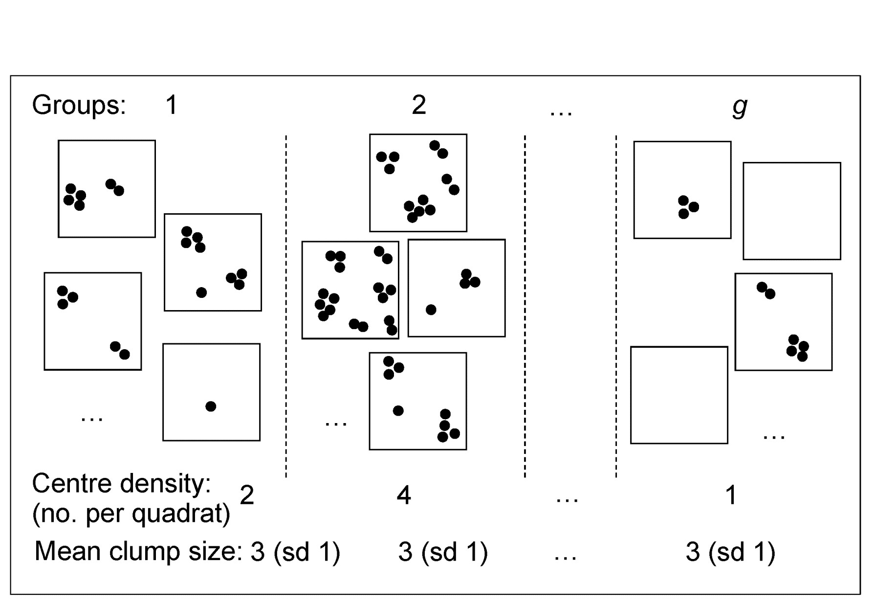
Fig 9.2 Simple graphic of generalised Poisson model for counts of a single species: centres of population are spatially random but with density varying across groups (sites/times/treatments). The distribution of the number of individuals(≥1) found at each centre is assumed constant across groups, though unknown.
Technically, for a particular species, if the number of centres in a replicate from group g has a Poisson distribution with mean $\nu _ g$ and the number of individuals at each centre has an unknown distribution with mean $\mu$ and variance $\sigma^2$, then $X _ j$, the count in the jth replicate from group g, has mean $\nu _ g \mu$ and variance $\nu _ g (\mu ^ 2 + \sigma ^ 2)$. Thus the index of dispersion D, the ratio of variance to mean counts for the group is $(\mu ^ 2 + \sigma ^ 2)/\mu$ and this is not a function of $\nu _ g$, i.e. D is the same for all groups, and an average D can be computed across groups (weighted, if replicates unbalanced). Dividing all counts by this average gives values which have the ‘Poisson-like’ property of variance $\approx$ mean.
The process is repeated for all species separately. Note that there is certainly no assumption that the clump size distribution is the same for all species, not even in distributional form: some species will be heavily clumped, others not at all, with all possibilities in between, but all are reduced by DW to giving (non-integral) abundances that are equally variable in relation to their mean, i.e. the unwanted contributions made by large but highly erratic counts are greatly down-weighted by their large dispersion indices.
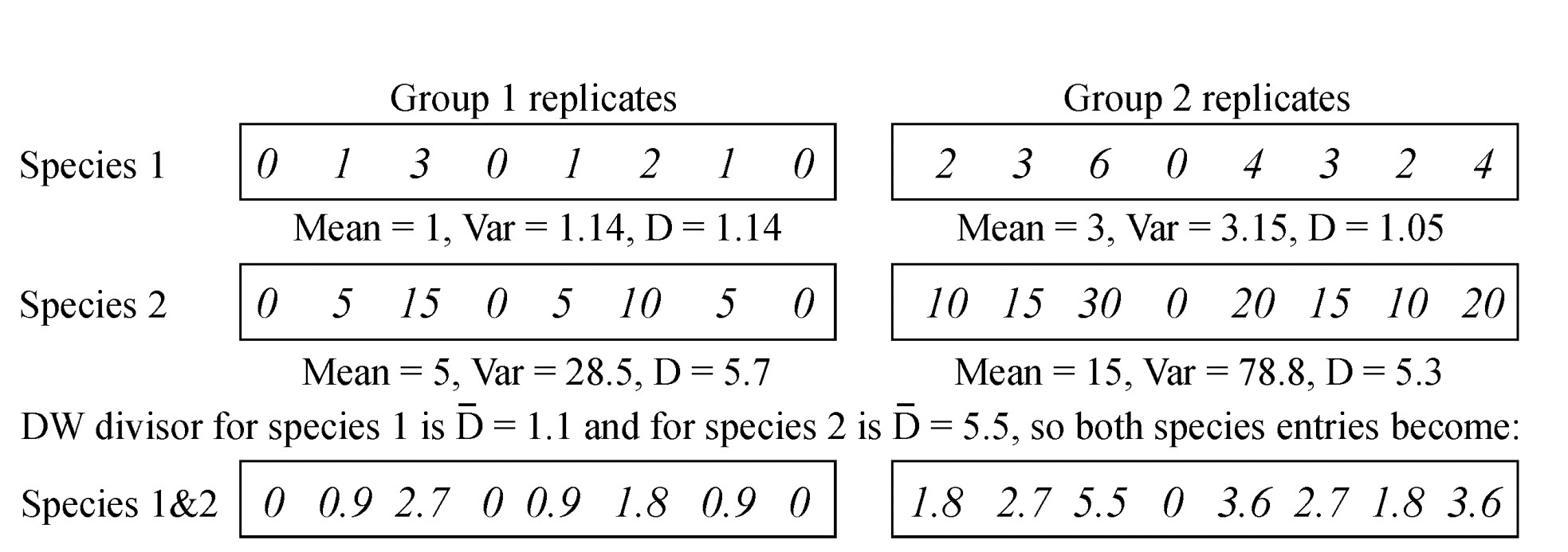
Table 9.5. Simple example of dispersion weighting (DW) on abundances from a matrix of two species sampled for two groups (e.g. sites/times), each of eight replicates. Prior to DW, species 2 would receive greater weight but its arrivals are clumped. After DW, the species have identical entries in the matrix.
One simple (over-simple) way of thinking of this is that we count clumps instead of individuals, and the calculation for such a simple hypothetical case is illustrated above. Here, there are two groups, with 8 replicates per group and two species. The individuals of species 1 arrive independently (the replicates show the Poisson-like property of variance $\approx$ mean) whereas species 2 has an identical pattern of arrivals but of clumps of 5 individuals at a time. Dividing through each set of species counts by the averaged dispersion indices (1.1 and 5.5 respectively) would reduce both rows of data to the same Poisson-like ‘abundances’.¶
However, DW is much more general than this simple case implies. The generalised Poisson model certainly includes the case of fixed-size clumps, and the even simpler case where the clump size is one, so that individuals arrive into the sample independently of each other, for which the counts are then Poisson and D=1 (DW applies no down-weighting). More realistically, it includes the Negative Binomial distribution as a special case, a distribution often advocated for fully parametric modelling of overdispersed counts (e.g. recently by Warton, Wright & Wang (2012) ). Such modelling needs the further assumption that the clump size distribution is of the same type for all species, namely Fisher’s log series. Also subsumed under DW are the Neyman type A (where the clump size distribution is also Poisson) and the Pólya-Aeppli (geometric clump size distribution) and many others.
Our approach here is to remain firmly distribution-free. In order to remove the large contributions that highly erratic (clumped) species counts can make to multivariate analyses such as the SIMPER procedure, it is not necessary (as Warton, Wright & Wang (2012) advocate) to throw out all the advantages of a fully multivariate approach to analysis, based on a biologically relevant similarity matrix, replacing them with what might be characterised as ‘parallel univariate analyses’. (This seems a classic case of ‘throwing the baby out with the bathwater’). Instead, it is simply necessary first to down-weight such species semi-parametrically, by dispersion weighting, which subsumes the negative binomial and many other commonly-used parametric models for overdispersed counts, and the (perceived§) problem disappears.
¶ In fact the counts for species 1 would not lead to rejection of the null hypothesis of independent random arrivals (D=1) in this case, using the permutation test discussed later, so no DW would be applied to species 1.
§ It is relevant to point out here that the later example (and much other experience) suggests that, whilst DW is more logically satisfactory than the cruder use of severe transformations for this purpose, the practical differences between analyses based on DW and on simple transforms are, at their greatest, only marginal. Since most of the 10,000+ papers using PRIMER software in its 20-year history have used transformed data (PRIMER even issues a warning if Bray-Curtis calculation has not been preceded by a transformation), Warton’s conclusions, largely based on analyses of untransformed data, that “hundreds of papers every year currently use methods [which] risk undesirable consequences” seem unjustified.
9.6 Example: Fal estuary copepods
Somerfield, Gee & Warwick (1994a) and Somerfield, Gee & Warwick (1994b) present biotic and environmental data from five creeks of the Fal estuary, SW England, whose sediments can contain high heavy metal levels resulting from historic tin and copper mining in the surrounding valleys ({f}, Fig. 9.3).
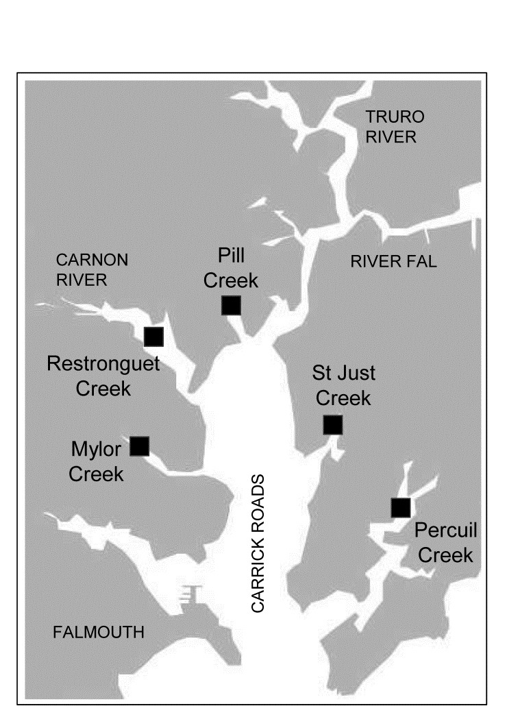
Fig. 9.3 Fal estuary copepods {f}. Five creeks sampled for meiofauna/macrofauna
Table 9.6. Fal estuary copepods {f}. Original counts from five replicate meiofaunal cores in each of two creeks (Mylor and Pill). Final three columns give the average dispersion index, its significance, and the divisor used to downweight each row (matrix is ordered by the latter) under the dispersion weighting procedure. Divisor=1 if permutation test does not give significant clumping for that species.
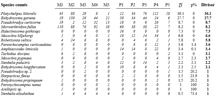
Here, only the infaunal copepod counts are analysed, from five replicate meiofaunal cores in each of two creeks (Mylor, M and Pill, P), subject to differing sediment concentrations of contaminants (Table 9.6). Species are listed in decreasing order of their average dispersion index $\overline{D}$ over the two groups, e.g. for the first species, Platychelipus littoralis, $D _ M =35.9$ and $D _ P =36.2$, giving average $\overline{D} = 36.1 $, the divisor for the first row of the matrix. This represents rather strong overdispersion for this species, as does the divisor $\overline{D} = 27.7$ for the second row, Enhydrosoma gariene. In fact, the highest counts in the matrix are found in these two species and, without DW, they would have played an influential role in determining the similarity measures input to the multivariate analyses. But their counts are not consistent over replicates, ranging from 1 to 88, 12 to 112, 19 to 130 etc, hence giving large dispersion indices (variance-to-mean ratios). The dispersion-weighted values, however, are now much lower, ranging only up to 3 or 4, and therefore strongly down-weighted in favour of more consistent species (over replicates), such as Microarthridion fallax. Its counts were initially similarly high but are subject to a much lower divisor, so this fourth row of the weighted matrix now ranges up to 13, giving it much greater prominence. Interestingly, even quite low-abundance species, such as the last in the list (Stenhelia elizabethae) will now make a significant contribution, because of its consistency; it does not get down-weighted at all, as the following permutation test shows.
Test for overdispersion
The final six species in the table exhibit no significant evidence of overdispersion at all, and their divisor is therefore 1. What is needed here to examine this is a test of the null hypothesis $D=1$ in all groups, and a relevant large-sample test is based on the standard Wald statistic for multinomial likelihoods (further details in Clarke, Chapman, Somerfield et al. (2006) ). This has the familiar chi-squared form, e.g. for Tachidius discipes how likely is it that observed counts for Mylor of 6, 2, 8, 0, 0 could arise from placing 16 individuals into 5 replicates independently and with equal probability, i.e. when the ‘expected’ values in each replicate are 3.2? Simultaneously, how likely is it that the two individuals from Pill both fall into the same replicate if they arrive independently (i.e. observed values are 0, 0, 0, 0, 2 and expected values 0.4 in each cell)? The usual chi-squared form $X ^2 = \sum \left[ (Obs - Exp)^2 / Exp \right] $ can be computed, but these are far from large samples so its distribution under the null hypothesis will only be poorly approximated by the standard $\chi ^ 2$ distribution on 8 df. Instead, in keeping with other tests of this manual, the null distribution is simply created by permutation: 16 and 2 individuals are randomly and independently placed into the first and second set of replicates, respectively, and $X ^ 2$ recalculated many times. For T. discipes the observed $X ^ 2$ is larger than any number of simulated ones and $D=1$ can be firmly rejected, so the divisor of 3.1 is used, but for the final 6 species $D=1$ is not rejected (at p=5% on this one-tailed test), and no down-weighting is carried out.
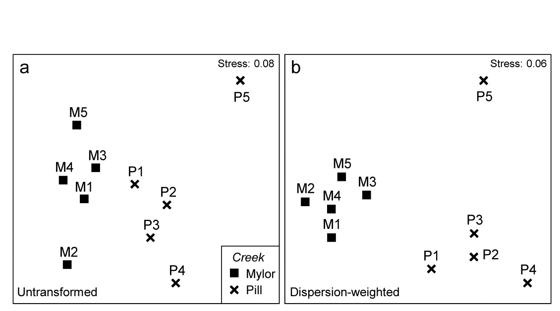
Fig 9.4 Fal estuary copepods {f}. MDS of copepod assemblages for 5 meiofaunal cores in each of two creeks (Mylor and Pill), from Bray-Curtis similarities on: a) untransformed counts; b) dispersion-weighted counts
Effect of dispersion weighting
The effect of DW on the multivariate analysis can be seen in Fig. 9.4, which contrasts the (non-metric) MDS plots from Bray-Curtis similarities based on untransformed and dispersion-weighted counts. A major difference is not observed, but there is a clear suggestion that the replicates within the M group in particular have tightened up, and the distinction between the two groups enhanced. The former is exactly what might be expected: by down-weighting species with large but erratic abundances in replicates we should be reducing the ‘noise’, allowing any ‘signal’ that may be there to be seen more clearly. But the latter cannot, and should not, be guaranteed. It is perfectly possible that when attention is focussed on the species that are consistent in replicates, they may display no change at all across groups – so be it. In fact, in this case, DW makes a sizeable difference to the ANOSIM test for the group effect, with the R statistic increasing from 0.41 to 0.71 after DW.
Shade plots to demonstrate matrix changes
The explanation, in terms of particular species, for changes seen in the multivariate analyses following DW, are well illustrated by simple shade plots (p7-7,
Clarke, Tweedley & Valesini (2014)
). For these visual representations of the data matrices, the intensity of grey shading is linearly proportional to the matrix entry, with white representing absence and full black the largest count (or weighted count) in the matrix, Fig. 9.5. Here, the species have been ordered according to a species clustering using the index of association on the original counts (equation 7.1), and the same species ordering is preserved for the shade plot under DW. It is readily seen that some of the less erratic species, such as M. fallax and S. elizabethae, do show a clear pattern of larger values at Mylor than Pill, and several other species which are not heavily down-weighted (Enhydrosoma longifurcatum, Amphiascoides limicola, Mesochra lilljeborgi) show the reverse pattern. The highly erratic species formerly given the most weight, P. littoralis and E. gariene, did not clearly distinguish the two creeks, so that their reduction in importance under DW has again, in this case, aided discrimination of the two groups.
Further DW issues
The DW procedure makes few assumptions about the data, but is derived from a model in which the degree of clumping, and thus the index of dispersion, of a particular species is constant across groups. In some cases this may well be a poor assumption, e.g. when impacts represented by a group structure affect both the propensity for that species to clump as well as the density of clump centres. Clearly, in that case, we must not use a different dispersion divisor D for each group; as earlier emphasised, doing different things for each group risks creating an artefactual group effect where none exists. Using an averaged index ($\overline{D}$) across groups might thus still provide a sensible ‘middle course’ in deciding how much weight to give to that species. Faced with the alternatives of doing no species weighting (so that erratic, clumped species dominate) or giving all species, abundant and rare, exactly the same weight (e.g. as in normalising the variables or the implicit standardisations of a Gower resemblance measure), DW may indeed be a robust general means of weighting species. As is seen later (e.g. Chapter 10 and 16 and Fig. 13.8), even quite major changes to the balance of information utilised from different species can have surprisingly little effect on a multivariate analysis, mainly because the latter typically uses only a small amount of information from each species and the same driving patterns are present in many species.
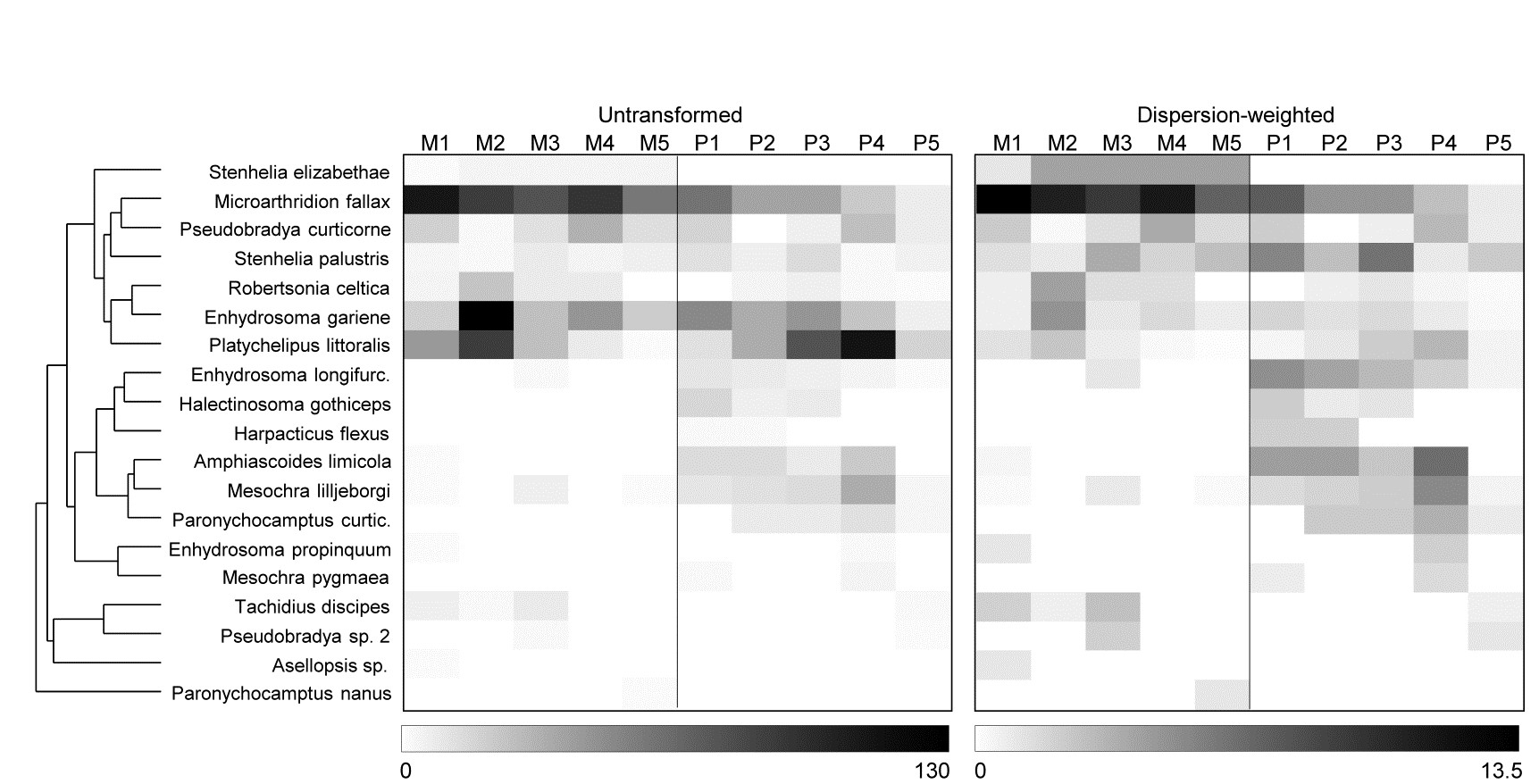
Fig. 9.5 Fal estuary copepods {f}. Shade plot, showing: left-hand, the untransformed counts of Table 9.6, represented by rectangles of linearly increasing grey scale (species clustering gives y-axis ordering); right-hand, the dispersion weighted values (maximum 13.4).
Clarke, Chapman, Somerfield et al. (2006) discuss further DW questions naturally arising. For example, should one upweight species that are significantly underdispersed, i.e. are territorially spaced, more evenly than expected under randomness, so that replicate counts are ‘too similar’ and chi-squared is significantly small? This is rarely observed, in the marine environment at least! Indeed, one of the beneficial side effects of applying DW is likely to be a clearer understanding of how a range of species are distributed in the environment, through histograms of dispersion indices calculated from all species in assemblages of different faunal types.
Also, how much more general can the DW idea be made? Clearly the test for D=1 is based on a realistic probability model for genuine counts but, if the testing structure is ignored, it would still logically make sense to apply downweighting by the variance-to-mean ratio for densities as well as counts, at least provided the adjustment from count to density was only of a modestly varying constant across samples. (A typical context might be where real counts from trawl samples are variably adjusted for modest differences in the volume of water filtered.) An extension to area cover data for rocky-shore or coral reef studies seems equally plausible. Here, the ‘counts’ can be thought of as number of grid points within a sampled area (one replicate) which fall on a particular species. If an individual algal or coral colony is larger than the grain of the grid points then the same colony will be ‘captured’ by several points, expressed as over-dispersion of the ‘counts’ from replicate to replicate (in the extreme, one species with an average area cover of 50% might vary from 100% in one replicate to 0% in the next, where another ubiquitous species, whose clump size is much smaller than the sampling grain, might record variation of only 40% to 60%). Relative down-weighting by dispersion indices then makes reasonable sense, and similar arguments could be adduced for biomass data of motile species. Larger-bodied species give greater ‘overdispersed’ biomass relative to smaller-bodied ones. In fact, by overlaying the previous model of real counts of organisms with a fixed body mass per individual (varying between species), relative downweighting by D works in exactly the same way as earlier, removing at the same time both greater clumping of individuals and the size differential between species, to leave a natural and robust weighting of the different species in subsequent multivariate analyses. It is, however, only relative D values that matter in all these cases; D=1 has no meaning outside the case of real counts.
DW vs. Transformation
DW is advocated above as an alternative to transformation, providing a more targeted way of dealing with large and highly variable counts in some species. The disadvantage of simple, severe transformations in this context (e.g. fourth root) is that, whilst effective in reducing the contribution of the erratic P. littoralis and E. gariene in the earlier example, they will also ‘squash’ consistent but low-abundance species, such as S. elizabethae, into a near presence/absence state. Nonetheless, simple transformations can be applied universally (e.g. without the need for replicates), and will often give similar results to DW. A fourth root transformation here actually leads to an even higher R value for the ANOSIM test for a group difference of 0.81, and the MDS plot, while similar, tightens up the Pill group by giving less emphasis to the lower total abundance at P5 than the other Pill creek sites; the latter was clearly seen in the shade plot, Fig. 9.5.
A shade plot for this fourth-root transformed matrix is shown in Fig. 9.6 (left-hand plot) and it is clear that the multivariate analyses will now mainly be driven by the differing presence/absence structure, with the originally important species playing a much smaller role (e.g. M. fallax now appears scarcely to differ between the two creeks).
DW and Transformation
However, the key step here is to realise that DW and transformation are not necessarily alternatives; it may be optimal to use them in combination. DW directly addresses the problem of undue emphasis being given to high abundance-high variance species, ensuring all weighted species values now have strictly comparable reliability. But DW does not address the primary motivation for transformations outlined in Chapter 2, that of better balancing the contributions from less abundant (and consistent) species with the more abundant (and now equally consistent) species. Not all high abundance species are erratic in replicates and, if they are, they may still have largely dominant values after DW has ensured their consistency. In short: DW is applied for statistical reasons but we may still need to transform further (after DW) for biological reasons, if we seek a ‘deeper rather than shallower’ view of the assemblage. That transform will likely now be less severe than if no DW had been carried out since it is no longer trying to address two issues at once. Here, the shade plot for DW followed by square root transformation is shown in Fig. 9.6 (right-hand plot) and this combination does actually give (marginally) the best separation of Mylor and Pill creeks in the multivariate analysis, amongst the analyses shown here, with R = 0.85.
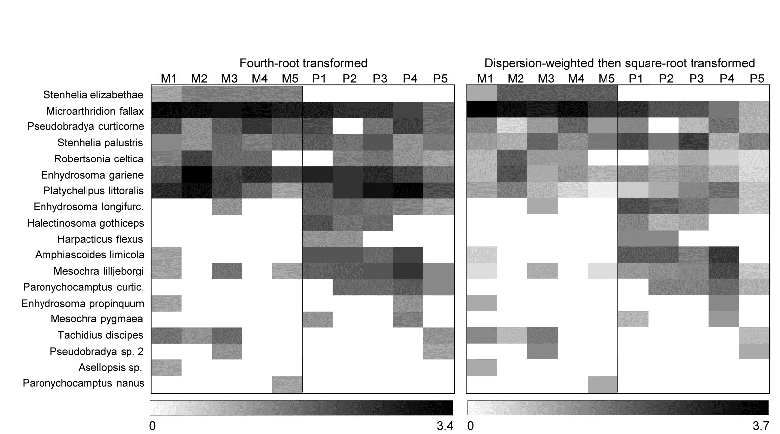
Fig. 9.6 Fal estuary copepods {f}. Shade plot, with linear grey scale for: left-hand, 4th-root transformed counts; right-hand, dispersion weighted values subsequently square-root transformed. Species order kept the same as in (untransformed) species clustering, Fig. 9.5.
This is not an uncommon finding. Clarke, Tweedley & Valesini (2014) describe the role of shade plots in assisting long-term choice of better transformation and/or DW strategies, and give examples. One is of fish studies in which highly schooling species, though heavily down-weighted by DW (by two orders of magnitude), remain dominant because they are consistently found in some quantity in all replicates. DW followed by mild transformation was transparently a better option than either DW or severe transformation on its own.
‘Long-term choice’ is an important phrase here: one must avoid the selection bias inherent in chasing the best combination of DW and transformation for each new study – ‘best’ in the sense of appealing most to our preconceptions of what the analysis should have demonstrated! Instead, the idea is to settle on a pre-treatment strategy to be used consistently in future for that faunal type in those sampling contexts.
9.7 Variability weighting
Hallett, Valesini & Clarke (2012) describe a similar idea to dispersion weighting for use when the data are continuous biological variables, such as diversity indices or other measures of ecological health of an assemblage. For such non-quantity data, for which zero plays no special role (and measures can be negative), variance-to-mean ratios are inappropriate. Instead, a natural weighting of indices in Euclidean distance calculation might be to divide each index by an average measure of its standard deviation (or range or IQ range) over replicates from each group. Indices with high replicate variability are then given less weight than more consistent ones. In some cases this may be preferable to normalising, which gives each index equal weight.