# 1.3 Example: Frierfjord macrofauna
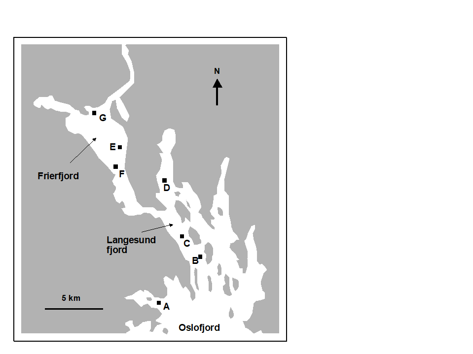
The first example is from the IOC/GEEP practical workshop on biological effects of pollutants ({{@224#bkmrk-bayne1988a}}), held at the University of Oslo, August 1986. This attempted to contrast a range of biochemical, cellular, physiological and community analyses, applied to field samples from potentially contaminated and control sites, in a fjordic complex (Frierfjord/Langesundfjord) linked to Oslofjord (***{F}***, Fig. 1.1). For the benthic macrofaunal component of this study ({{@224#bkmrk-gray1988a}}), four replicate 0.1m2 Day grab samples were taken at each of six sites (A-E and G, Fig 1.1) and, for each sample, organisms retained on a 1.0 mm sieve were identified and counted. Wet weights were determined for each species in each sample, by pooling individuals within species.
[](https://learninghub.primer-e.com/uploads/images/gallery/2022-02/fig1-1.png)
***Fig. 1.1. Frierfjord, Norway {F}.** Benthic community sampling sites (A-G) for the IOC/GEEP Oslo Workshop; site F omitted for macrobenthos.*
[](https://learninghub.primer-e.com/uploads/images/gallery/2022-02/OoRfig1-2.png)
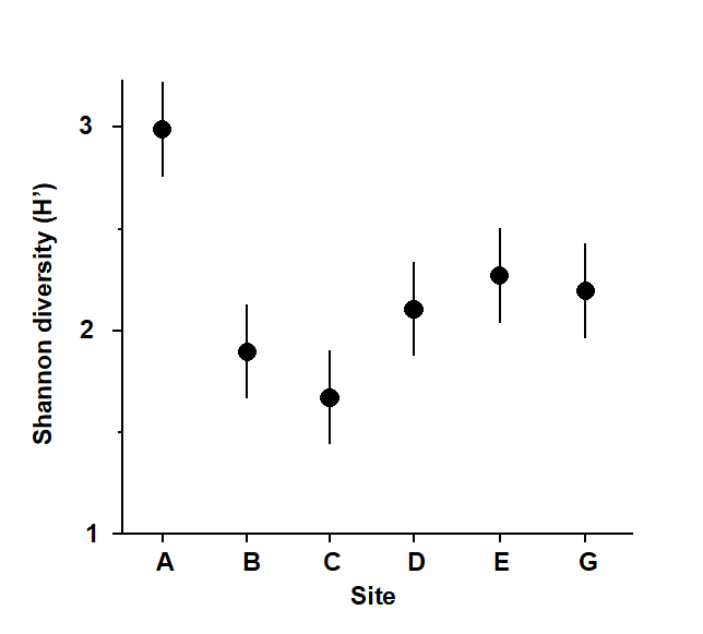
***Fig. 1.2. Frierfjord macrofauna {F}.** Means and 95% confidence intervals for Shannon diversity (H'), from four replicates at each of six sites (A-E, G).*
Part of the resulting data matrix can be seen in Table 1.2: in total there were 110 different taxa categorised from the 24 samples. Such matrices (abundance, *A*, and/or biomass, *B*) are the starting point for the biotic analyses of this manual, and this example is typical in respect of the relatively high ratio of species to samples (always >> 1) and the prevalence of zeros. Here, as elsewhere, even an undesirable reduction to the 30 ‘most important’ species (see [Chapter 2](https://learninghub.primer-e.com/books/change-in-marine-communities/chapter/chapter-2-simple-measures-of-similarity-of-species-abundance-between-samples)) leaves more
than 50% of the matrix consisting of zeros. Standard multivariate normal analyses (e.g. {{@224#bkmrk-mardia1979a}}) of these counts are clearly ruled out; they require both that the number of species (variables) be small in relation to the number of samples, and that the abundance or biomass values are transformable to approximate normality: neither is possible.
***Table 1.2. Frierfjord macrofauna {F}.** Abundance and biomass matrices (part only) for the 110 species in 24 samples (four replicates at each of six sites A-E, G); abundance in numbers per 0.1m2, biomass in mg per 0.1m2.*
|**Species**|` `**Samples**|
| :- | :-: |
|` `|A1|A2|A3|A4|B1|B2|B3|B4|
|:-|:-: | :-: | :-: | :-: | :-: | :-: | :-: | :-:|
|**Abundance**|||||||||
|*Cerianthus lloydi*|*0*|*0*|*0*|*0*|*0*|*0*|*0*|*0*|
|*Halicryptus sp.*|*0*|*0*|*0*|*1*|*0*|*0*|*0*|*0*|
|*Onchnesoma*|*0*|*0*|*0*|*0*|*0*|*0*|*0*|*0*|
|*Phascolion strombi*|*0*|*0*|*0*|*1*|*0*|*0*|*1*|*0*|
|*Golfingia sp.*|*0*|*0*|*0*|*0*|*0*|*0*|*0*|*0*|
|*Holothuroidea*|*0*|*0*|*0*|*0*|*0*|*0*|*0*|*0*|
|*Nemertina, indet.*|*12*|*6*|*8*|*6*|*40*|*6*|*19*|*7*|
|*Polycaeta, indet.*|*5*|*0*|*0*|*0*|*0*|*0*|*1*|*0*|
|*Amaena trilobata*|*1*|*1*|*1*|*0*|*0*|*0*|*0*|*0*|
|*Amphicteis gunneri*|*0*|*0*|*0*|*0*|*4*|*0*|*0*|*0*|
|*Ampharetidae*|*0*|*0*|*0*|*0*|*1*|*0*|*0*|*0*|
|*Anaitides groenl.*|*0*|*0*|*0*|*1*|*1*|*0*|*0*|*0*|
|*Anaitides sp.*|*0*|*0*|*0*|*0*|*0*|*0*|*0*|*0*|
|. . . . |||||||||
|**Biomass**|||||||||
|*Cerianthus lloydi*|*0*|*0*|*0*|*0*|*0*|*0*|*0*|*0*|
|*Halicryptus sp.*|*0*|*0*|*0*|*26*|*0*|*0*|*0*|*0*|
|*Onchnesoma*|*0*|*0*|*0*|*0*|*0*|*0*|*0*|*0*|
|*Phascolion strombi*|*0*|*0*|*0*|*6*|*0*|*0*|*2*|*0*|
|*Golfingia sp.*|*0*|*0*|*0*|*0*|*0*|*0*|*0*|*0*|
|*Holothuroidea*|*0*|*0*|*0*|*0*|*0*|*0*|*0*|*0*|
|*Nemertina, indet.*|*1*|*41*|*391*|*1*|*5*|*1*|*2*|*1*|
|*Polycaeta, indet.*|*9*|*0*|*0*|*0*|*0*|*0*|*0*|*0*|
|*Amaena trilobata*|*144*|*14*|*234*|*0*|*0*|*0*|*0*|*0*|
|*Amphicteis gunneri*|*0*|*0*|*0*|*0*|*45*|*0*|*0*|*0*|
|*Ampharetidae*|*0*|*0*|*0*|*0*|*0*|*0*|*0*|*0*|
|*Anaitides groenl.*|*0*|*0*|*0*|*7*|*11*|*0*|*0*|*0*|
|*Anaitides sp.*|*0*|*0*|*0*|*0*|*0*|*0*|*0*|*0*|
|. . . .|||||||||
As discussed above, one easy route to simplification of this ***high-dimensional*** (multi-species) complexity is to reduce each matrix column (sample) to a single univariate description. Fig. 1.2 shows the results of computing the Shannon diversity (H', see [Chapter 8](https://learninghub.primer-e.com/books/change-in-marine-communities/chapter/chapter-8-diversity-measures-dominance-curves-and-other-graphical-analyses)) of each sample**¶**, and plotting for each site the mean diversity and its 95% confidence interval, based on a pooled estimate of variance across all sites from the ANOVA table, [Chapter 6](https://learninghub.primer-e.com/books/change-in-marine-communities/chapter/chapter-6-testing-for-differences-between-groups-of-samples). (An analysis of the type outlined in [Chapter 9](https://learninghub.primer-e.com/books/change-in-marine-communities/chapter/chapter-9-transformations-and-dispersion-weighting) shows that prior transformation of H' is not required; it already has approximately constant variance across the sites, a necessary prerequis�ite for standard ANOVA). The most obvious feature of Fig. 1.2 is the relatively higher diversity at the ***control***/***reference*** location, A.
---
**¶** *Using the PRIMER DIVERSE routine.*