# 6.1 Univariate tests and multivariate tests
Many community data sets possess some *a priori* defined structure within the set of samples, for exam�ple there may be replicates from a number of differ�ent sites (and/or times). A pre-requisite to interpreting community differences between sites should be a demonstration that there *are* statistically significant differences to interpret.
### Univariate tests
When the species abundance (or biomass) information in a sample is reduced to a single index, such as Shannon diversity (see [Chapter 8](https://learninghub.primer-e.com/books/change-in-marine-communities/chapter/chapter-8-diversity-measures-dominance-curves-and-other-graphical-analyses)), the existence of replicate samples from each of the groups (sites/times etc.) allows formal statistical treatment by analysis of variance (ANOVA). This requires the assumption that the univariate index is normally distributed and has constant variance across the groups, conditions which are normally not difficult to justify (perhaps after transformation, see [Chapter 9](https://learninghub.primer-e.com/books/change-in-marine-communities/chapter/chapter-9-transformations-and-dispersion-weighting)). A so-called ***global test*** of the ***null hypothesis*** (H$ _ o$), that there are no differences between groups, involves computing a particular ratio of variability in the group means to variability among replicates within each group. The resulting ***F statistic*** takes values near 1 if the null hypothesis is true, larger values indicating that H$ _ o$ is false; standard tables of the *F* distribution yield a significance level *(p)* for the observed *F* statistic. Broadly speaking, *p* is interpreted as the probability that the group means we have observed (or a set of means which appear to differ from each other to an even greater extent) could have occurred if the null hypothesis H$_ o$ is actually true.
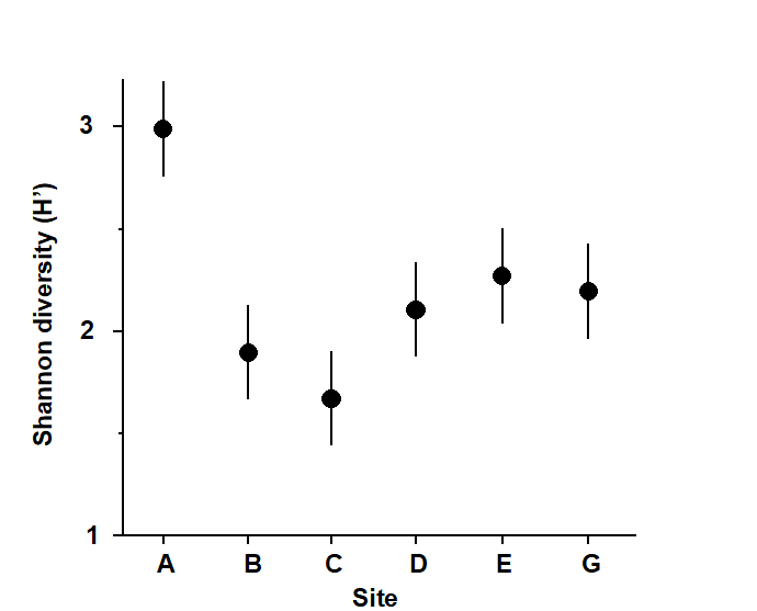
Fig.6.1 and Table 6.1 provide an illustration, for the 6 sites and 4 replicates per site of the Frierfjord macro�fauna samples. The mean Shannon diversity for the 6 sites is seen in Fig.6.1, and Table 6.1 shows that the *F* ratio is sufficiently high that the probability of observing means as disparate as this by chance is *p*<0.001 (or *p*<0.1%), if the true mean diversity at all sites is the same. This is deemed to be a sufficiently unlikely chance event that the null hypothesis can safely be rejected. Convention dictates that values of *p*<5% are sufficiently small, *in a single test*, to discount the possibility that H$_ o$ is true, but there is nothing sacrosanct about this figure: clearly, values of *p* = 4% and 6% should result in the same inference. It is also clear that repeated significance tests, each of which has (say) a 5% possibility of describing a chance event as a real difference, will cumulatively run a much greater risk of drawing at least one false inference. This is one of the (many) reasons why it is not usually appropriate to handle a multi-species matrix by performing an ANOVA on each species in turn. (Further reasons are the complexities of dependence between species and the general inappropriateness of normality assumptions for abundance-type data).
[](https://learninghub.primer-e.com/uploads/images/gallery/2022-02/ch6fig6-1.png)
***Fig. 6.1. Frierfjord macrofauna {F}.** Means and 95% confid�ence intervals of Shannon diversity (H$^\prime$) at the 6 field sites (A-E, G) shown in Fig. 1.1.*
Fig. 6.1 shows the main difference to be a higher diversity at the outer site, A. The intervals displayed are ***95% confidence intervals*** for the true mean diversity at each site; note that these are of equal width because they are based on the assumption of constant variance, that is, they use a pooled estimate of replication variability from the residual mean square in the ANOVA table.
***Table 6.1. Frierfjord macrofauna {F}.** ANOVA table showing rejection (at a significance level of 0.1%) of the global hypothesis of ‘no site-to-site differences’ in Shannon diversity (H’).*
||Sum of squares|Deg. of freedom|Mean Square|F ratio|Sig. level|
| :- | :- | :- | :- | :- | :- |
|||||||
|Sites|*3.938*|` `*5*|*0.788*|*15.1*|*< 0.1%*|
|Residual|*0.937*|*18*|*0.052*|||
|Total|*4.874*|*23*||||
Further details of how confidence intervals are deter�mined, why the ANOVA *F* ratio and *F* tables are defined in the way they are, how one can allow to some extent for the repeated significance tests in pairwise comparisons of site means etc, are not pursued here. This is the ground of basic statistics, covered by many standard texts, for example {{@224#bkmrk-sokal1981a}}, and such computations are available in all general-purpose statistics packages. This is not to imply that these concepts are elementary; in fact it is ironic that a proper understanding of *why* the univariate *F* test works requires a level of mathemat�ical sophistication that is not needed for the simple permutation approach to the analogous global test for differences in *multivariate* structure between groups, outlined below.
### Multivariate tests
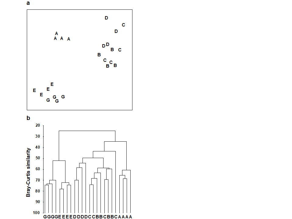
One important feature of the multivariate analyses described in earlier chapters is that they in no way utilise any known structure among the samples, e.g. their division into replicates within groups. (This is in contrast with Canonical Variate Analysis, for example, which deliberately seeks out ordination axes that, in a certain well-defined sense, best separate out the known groups; e.g. {{@224#bkmrk-mardia1979a}}). Thus, the ordination and dendrogram of Fig 6.2, for the Frierfjord macrofauna data, are constructed only from the pairwise similarities among the 24 samples, treated simply as numbers 1 to 24. By superimposing the group (site) labels A to G on the respective replicates it becomes immediately apparent that, for example, the 4 replicates from the outer site (A) are quite different in community composition from both the mid-fjord sites B, C and D and the inner sites E and G. A statistical test of the hypothesis that there are no site-to-site differences overall is clearly un�necess�ary, though it is less clear whether sufficient evidence exists to assert that B, C and D differ.
[](https://learninghub.primer-e.com/uploads/images/gallery/2022-02/ch6fig6-2.png)
***Fig. 6.2 Frierfjord macrofauna {F}**. a) MDS plot, b) dendro�gram, for 4 replicates from each of the 6 sites (A-E and G), from Bray Curtis similarities computed for $\sqrt{} \sqrt{}$-transformed species abundances (MDS stress = 0.05).*
This simple structure of groups, and replicates within groups, is referred to as a ***1-way*** ***layout***, and it was seen above that 1-way ANOVA would provide the appropriate testing framework *if* the data were univariate (e.g. diversity or total abundance across all species). There *is* an analogous multivariate analysis of variance (MANOVA, e.g. {{@224#bkmrk-mardia1979a}}), in which the *F* test is replaced by a test known as Wilks’ $\Lambda$, but its assumptions will never be satisfied for typical multi-species abundance (or biomass) data. This is the problem referred to in the earlier chapters on choosing similarities and ordination methods; there are typically many more species (variables) than samples and the probability distribution of counts could never be reduced to approximate (multivariate) normality, by any transformation, because of the dominance of zero values. For example, for the Frierfjord data, as many as 50% of the entries in the species/samples matrix are zero, even after reducing the matrix to only the 30 most abundant species!
A valid test can instead be built on a simple non-parametric permutation procedure, applied to the (rank) similarity matrix underlying the ordination or classification of samples, and therefore termed an ANOSIM test (***analysis of similarities***)¶, by analogy with the acronym ANOVA (analysis of variance). The history of such permutation tests dates back to the epidemiological work of {{@224#bkmrk-mantel1967a}}, and this is combined with a general randomization approach to the generation of significance levels ({{@224#bkmrk-hope1968a}}). In the context below, it was described by {{@224#bkmrk-clarke1988b}}.
---
¶ *The PRIMER ANOSIM routine covers tests for replicates from 1-, 2- and 3-way (nested or crossed) layouts in all combinations. In 2- or 3-way crossed cases without replication, a special form of the ANOSIM routine can still provide a (rather different style of) test; all the possibilities are worked through in this chapter.*