Chapter 2: Tests of homogeneity of dispersions (PERMDISP)
Key reference Method: Anderson (2006)
- 2.1 General description
- 2.2 Rationale
- 2.3 Multivariate Levene’s test (Bumpus’ sparrows)
- 2.4 Generalisation to dissimilarities
- 2.5 $P$-values by permutation
- 2.6 Test based on medians
- 2.7 Ecological example (Tikus Island corals)
- 2.8 Choice of measure
- 2.9 Dispersion as beta diversity (Norwegian macrofauna)
- 2.10 Small sample sizes
- 2.11 Dispersion in nested designs (Okura macrofauna)
- 2.12 Dispersion in crossed designs (Cryptic fish)
- 2.13 Concluding remarks
2.1 General description
Key reference
-
Method:
Anderson (2006)
PERMDISP is a routine for testing the homogeneity of multivariate dispersions on the basis of any resemblance measure. The test is a dissimilarity-based multivariate extension of Levene’s test ( Levene (1960) ), following the ideas of van Valen (1978) , O’Brien (1992) and Manly (1994) , who used Euclidean distances. In essence, the test uses the ANOVA F statistic to compare (among different groups) the distances from observations to their group centroid. The user has the choice of whether to perform the test on the basis of distances to centroids or distances to spatial medians ( Gower (1974) ). The user also has the choice either to use traditional tables or to use permutation of appropriate residuals (either least-squares residuals if centroids are used or least-absolute-deviation residuals if spatial medians are used) in order to obtain P-values.
2.2 Rationale
There are various reasons why one might wish to perform an explicit test of the null hypothesis of no differences in the within-group multivariate dispersion among groups. First, such a test provides a useful logical complement to the test for location differences that are provided by PERMANOVA. As pointed out in chapter 1, PERMANOVA, like ANOSIM, is sensitive to differences in multivariate dispersion among groups (e.g., see Fig. 1.6). In fact, the logic of the partitions of variability for all of the ANOVA designs in chapter 1 dictates that the multivariate dispersions of the residuals should be homogeneous, as should also be the dispersions of levels for random factors in nested designs and mixed models. A significant result for a given factor from PERMANOVA could signify that the groups differ in their location (Fig. 2.1b), in their dispersion (Fig. 2.1c) or some combination of the two (Fig. 2.1d). An analysis using PERMDISP focuses only on dispersion effects, so teases out this part of the null hypothesis (equal dispersions) on its own, perhaps as a prelude to a PERMANOVA analysis, analogous to a univariate test for homogeneity prior to fitting ANOVA models.

Fig. 2.1. Schematic diagram showing two groups of samples in a bivariate system (two dimensions) that (a) do not differ in either location or dispersion, (b) differ only in their location in multivariate space, (c) differ only in their relative dispersions and (d) differ in both their location and in their relative dispersion.
Of course, the other reason for applying a test of dispersion is because specific hypotheses of interest may demand such an analysis in its own right. There are many situations in ecology for which changes in the variability of assemblages are of direct importance. For example, increases or decreases in the multivariate dispersion of ecological data has been identified as a potentially important indicator of stress in marine communities ( Warwick & Clarke (1993) , Chapman, Underwood & Skilleter (1995) ).
2.3 Multivariate Levene’s test (Bumpus’ sparrows)
Levene (1960) proposed doing an analysis of variance (ANOVA) on the absolute values of deviations of observations from their group mean. A multivariate analogue was described by van Valen (1978) and given in Manly (1994) , based on distances. Let $y _{ij}$ be a vector of p response variables for the jth observation in the ith group and let $\bar{y} _i$ be the centroid vector for group i, then the distance between each observation and its group centroid is a single value that can be denoted by $z _{ij}$. This is visualised easily in the case of two variables (two dimensions), as shown in Fig. 2.2 for the case of 2 groups. Once a value of z is calculated for each observation, this is treated as a univariate variable and the test consists of doing a traditional ANOVA comparing the values of z among the groups. The central idea here is that if the groups differ in their within-group dispersions, then the values of z (on average) will differ among the groups. Note that if Euclidean distance is used and there is only one variable, then the PERMDISP test is equivalent to the traditional univariate Levene’s test.
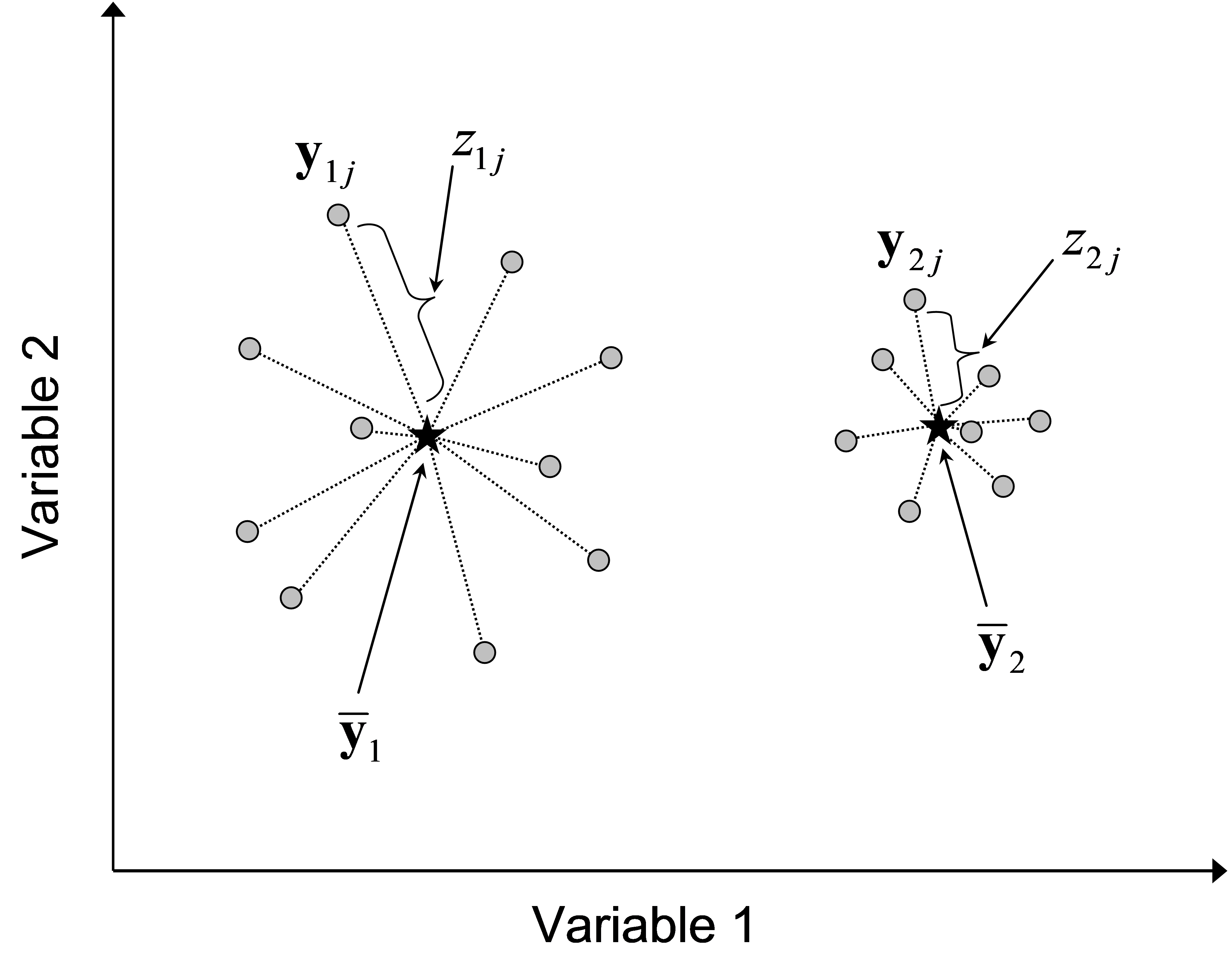
Fig. 2.2. Schematic diagram in a bivariate (two-variable) system showing the distances to centroids (z’s) for each of two groups, as used in a multivariate analogue to Levene’s test.
An example is provided by Manly (1994) who analysed the morphometric characteristics of sparrows from data due to Bumpus (1898) . It was hypothesised that stabilising selection acting on organisms should reduce the multivariate heterogeneity of their morphometric characteristics. The data consist of p = 5 morphometric variables (total length, alar extent, length of beak/head, length of humerus and length of keel of sternum, all in mm) from each of N = 49 female sparrows. Twenty-one of the sparrows died in a storm and twenty-eight survived. Of central interest is the question: are the morphologies of the sparrows that died more variable than for those that survived? That is, are sparrows with morphologies distant from the “norm” or “average” sparrow more likely to have died?
The data are located in the file spar.pri in the ‘BumpSpar’ folder of the ‘Examples add-on’ directory. Observations on the raw data (e.g., using a draftsman plot) reveal that the variables are quite well-behaved (approximately normal), as is usual with morphometric data, and that they are correlated with one another. A PCA (principal components analysis) would be a good idea for ordination (see chapter 4 of Clarke & Warwick (2001) for details). These variables are, however, on quite different measurement scales and so should be normalised before further analysis. Choose Analyse > Pre-treatment > Normalise variables. Next, for the normalised data, choose Analyse > PCA. The first two principal components account for about 83% of the total variation across the 5 variables and are shown in Fig. 2.3. There appears to be slightly greater variation in morphological characteristics (i.e. a slightly greater spread of points) for the sparrows that died compared to the ones that survived, but the extent of such differences, if any, can be difficult to discern in a reduced-space ordination plot.

Fig. 2.3. PCA ordination of Bumpus’ sparrows on the basis of 5 normalised morphometric variables.
To test the null hypothesis of no difference in dispersion between the two groups (Fig. 2.4), begin by selecting the normalised data and then choose Analyse > Resemblance > (Analyse between •Samples) & (Measure •Euclidean distance). From the resemblance matrix, choose PERMANOVA+ > PERMDISP > (Group factor: Group) & (Distances are to •Centroids) & (P-values are from •Tables). There is some evidence to suggest a difference in dispersion between the two groups, although the P-value obtained is borderline (F = 3.87, P = 0.055, Fig. 2.4).
 Fig. 2.4. Test of homogeneity of dispersions for Bumpus’ sparrow data on the basis of Euclidean distances of normalised variables using PERMDISP.
The output provides not only the value of the F ratio and its associated P-value, but also gives the mean and standard error for the z values in each group. These values are interpretable on the scale of the original resemblance measure chosen. Thus, in the present case, the average distance-to-centroid in the Euclidean space of the normalised morphometric variables is 1.73 for the sparrows that survived and 2.23 for the sparrows that died. The mean distance-to-centroid (± 1 standard error) might be usefully plotted in the case of there being many groups to compare (e.g., Anderson (2006) ). The individual z values obtained for each observation (from which the mean and standard errors are calculated) will also be provided in the results file if one chooses ($\checkmark$Output individual deviation values) in the PERMDISP dialog box (Fig. 2.4).
2.4 Generalisation to dissimilarities
Of course, in many applications that we will encounter (especially in the case of community data), the Euclidean distance may not be the most appropriate measure for the analysis. What we require is a test of homogeneity of dispersions that will allow any resemblance measure to be used. There are (at least) two potential problems to overcome in order to proceed. First, there is the issue that the centroids in the space of the dissimilarity (or similarity) measure chosen are generally not the same as the vector of arithmetic averages taken for each of the original variables (which is what we would normally calculate as being in the “centre” of the cloud in Euclidean space). Therefore, it is not appropriate to calculate (say) the Bray-Curtis dissimilarity between an observation and its group centroid when the centroid has simply been calculated as an arithmetic average. What is needed, instead, is the “centre” of the cloud of points for each group in Bray-Curtis (rather than Euclidean) space (or in whatever space has been defined by the dissimilarity measure of choice for the particular analysis) .
The solution to this is to place the points into a Euclidean space in such a way so as to preserve all of the original inter-point dissimilarities. This is achieved through the use of a method called principal coordinates analysis (PCO, see chapter 3), described by Torgerson (1958) and Gower (1966) . In essence, PCO generates a new set of variables (principal coordinate axes) in Euclidean space from the dissimilarity matrix ( Legendre & Legendre (1998) ). Usually, PCO is used for ordination (see chapter 3), and in this case only the first two or three PCO axes are drawn and examined. However, the full analysis actually generates a larger number of PCO axes (usually up to N – 1, where N is the total number of samples). All of the PCO axes taken together can be used to re-create the full set of inter-point resemblances, but in Euclidean space. More particularly (and here is what interests us for the moment), if we calculate the Euclidean distance between, say, sample 1 and sample 2, using all of the PCO axes, then this will be equal to the dissimilarity calculated between those same two sample points using the original variables52. Thus, any calculation that would be appropriate in a Euclidean context (such as calculating centroids as arithmetic averages), can be achieved in a non-Euclidean (dissimilarity) space by performing the operation on PCO axes from the resemblance matrix.
This means that we can proceed with the following steps in order to obtain the correct values for z in more general (non-Euclidean distance) cases: (i) calculate inter-point dissimilarities, using the resemblance measure of choice; (ii) do a PCO of this dissimilarity matrix; (iii) calculate centroids (arithmetic averages) of groups using the full set of PCO axes; and (iv) calculate the Euclidean distance from each point to its group centroid using the PCO axes. These then correspond to the dissimilarity from each point to its group centroid in the space of the chosen resemblance measure. The PERMDISP routine indeed follows these four steps (see Anderson (2006) for more details) in order to calculate appropriate z values for the test of homogeneity of dispersions on the basis of any dissimilarity measure53.
52 The distances obtained from the PCO axes must be calculated by first keeping the axes that correspond to the negative and the positive eigenvalues separate. These two parts are then brought together to calculate the final distance by taking the square root of the difference in two terms: the positive sum of squares and the absolute value of the negative sum of squares. This will result in a real (non-imaginary) value provided the positive portion exceeds the negative portion. See Anderson (2006) and chapter 3 of this manual for more details.
53 The use of PCO axes to calculate centroids and the use of permutation methods to obtain P-values are two important ways that the method implemented by PERMDISP differs from the method proposed by Underwood & Chapman (1998) .
2.5 $P$-values by permutation
The other hurdle that must be cleared is to recognise that, in line with the philosophy of all of the routines in the PERMANOVA+ add-on, we have no particular reason to assume that the distribution of the z’s will be necessarily normal. Yet, to use tabled P-values for Fisher’s F distribution requires this assumption to be made. Of course, we wish to cater for any situation where the z’s may be non-normal. This can be achieved by using a permutation procedure.
Note that, unlike the PERMANOVA one-way analysis, it does not make sense to simply permute the labels randomly among the groups to test the null hypothesis of homogeneity. This is because such permutations will cause potential differences in location among the groups to suddenly be included as part of the “within-group” measures. However, differences in location do not form part of the null hypothesis and so it is not logical to be mixing samples together from groups having different locations as possible alternative outcomes if the null hypothesis were true. Before proceeding, the observations from different groups must therefore be centered onto a common group centroid. In other words, it is the residuals obtained after removing any location differences that are actually exchangeable under the null hypothesis of homogeneity of dispersions. Permutation of residuals ( Freedman & Lane (1983) ) is an approach that has been demonstrated to have good asymptotic and empirical properties ( Anderson & Legendre (1999) , Anderson & Robinson (2001) ). PERMDISP uses permutation of residuals (i.e., permutation of samples among groups after centering all groups onto a common location) in order to generate P-values for the test.
2.6 Test based on medians
Levene’s test (for univariate data) can be made more robust (i.e. less affected by outliers) by using deviations from medians rather than deviations from means ( Brown & Forsythe (1974) , Conover, Johnson & Johnson (1981) ). However, for multivariate data, there is more than one way to define a median ( Haldane (1948) , Gower (1974) , Brown (1983) ). One definition of a median for multivariate data is the vector of medians for each individual variable (e.g., O’Brien (1992) , Manly (1994) ). Another possibility is to invoke a spatial concept for the median as the point in the multivariate cloud which minimises the sum of the distances from each observation to that point, called the ‘mediancentre’ by Gower (1974) . This spatial median is invariant to rotational changes in the axes, a quality which is not shared by the vector of medians of individual variables. This invariance to rotation is important for our purposes here, where PCO axes (which can involve rotations of the original data cloud) might be used, so PERMDISP (optionally) uses spatial medians.
An analysis that calculates the z values as deviations from spatial medians (rather than centroids) will clearly be less affected by outliers, so will tend to be more robust if the distribution of points in the data cloud is highly skewed for some reason. PERMDISP provides an option to perform the test based on medians rather than centroids: simply choose (Distances are to •Medians) in the PERMDISP dialog box (Fig. 2.4). Note that the residuals which are permuted for the test based on medians are not the least-squares (LS) residuals (as are used for the test on the basis of centroids). Instead, the multivariate analogue of least absolute deviation (LAD) residuals (e.g., Cade & Richards (1996) ) are permuted instead. That is, the groups are first centered on to a common spatial median before proceeding with the permutations.
Relevant aside: If you have a single variable and the analysis is based on a Euclidean distance matrix, then PERMDISP using centroids and tables will give Levene’s ( Levene (1960) ) original univariate test, while PERMDISP using medians and tables will give the modification of Levene’s test proposed by Brown & Forsythe (1974) 54 for univariate data.
Recommendation: Simulations with multivariate ecological datasets indicated that the test using PERMDISP on the basis of distances to centroids, with P-values obtained using permutations, gave the best overall results (in terms of type I error and power, Anderson (2006) ). These are thus the default options for the routine.
54 The version of Levene’s test used most commonly and available in many statistical computer packages is this version based on medians.
2.7 Ecological example (Tikus Island corals)
An ecological example of the test for homogeneity is provided by considering a study by Warwick, Clarke & Suharsono (1990) on coral assemblages from South Tikus Island, Indonesia. Percentage cover was measured along 10 transects for 75 species of coral in each of several years (1981-1988) which spanned an El Niño weather event occurring in 1982-83. For simplicity, we shall consider here only the years 1981, 1983 and 1985. The data are located in the file tick.pri in the ‘Corals’ folder of the ‘Examples v6’ directory for PRIMER. Open up the file in PRIMER and select only the years 81, 83 and 85 from the dialog box obtained by choosing Select > Samples > •Factor levels > Factor name: Year and clicking on the ‘Levels’ button and picking out these years. An MDS plot of these samples on the basis of the Bray-Curtis measure (Fig. 2.5) shows a clear pattern of apparently much greater dispersion (variability) among the samples obtained in 1983, right after the El Niño event, with relatively less dispersion among samples obtained either before (1981) or two years after (1985).
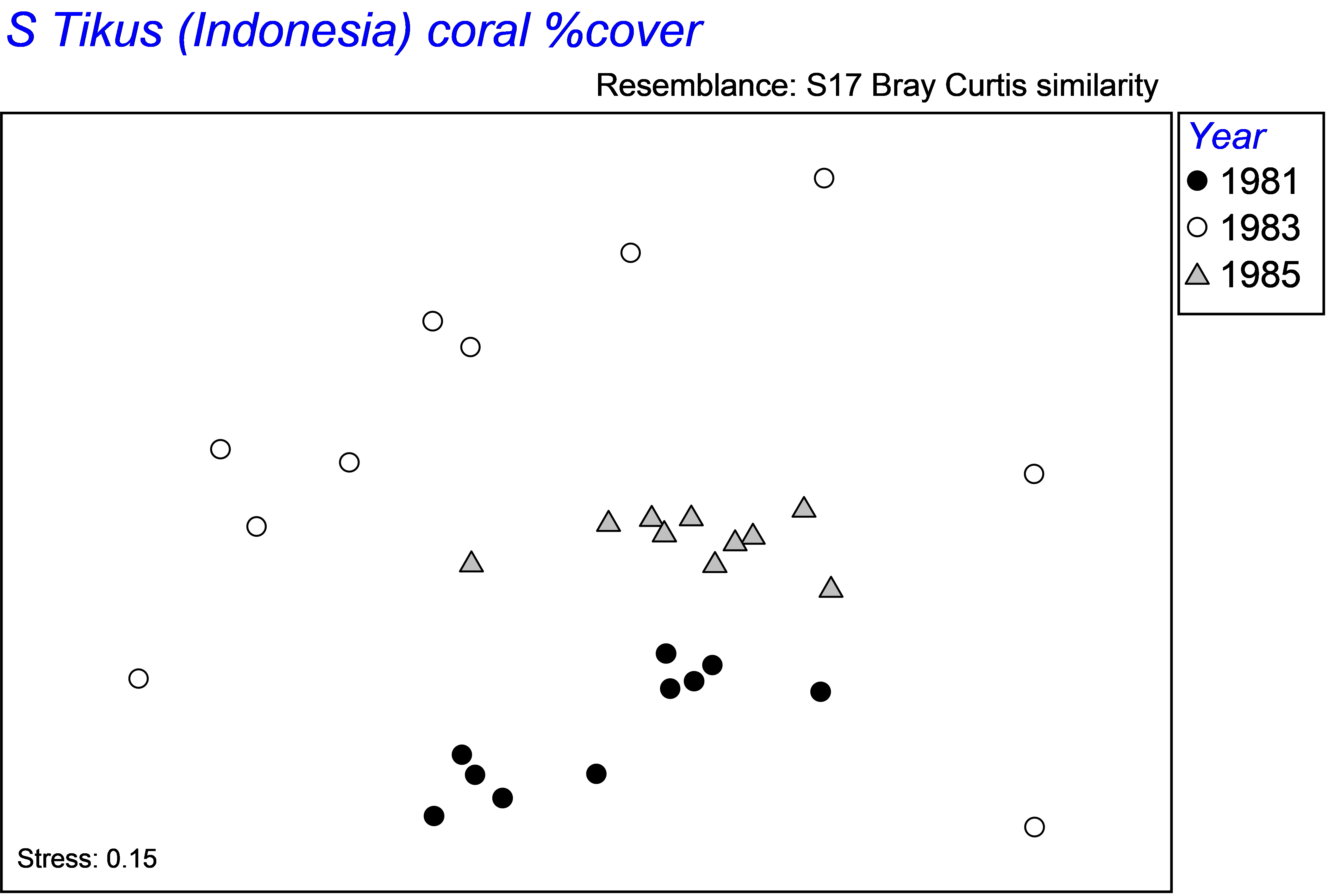
Fig. 2.5. MDS of coral assemblages from South Tikus Island in each of three years based on Bray-Curtis.
To perform the test for homogeneity of dispersions for these data (Fig. 2.6), click on the resemblance matrix and choose PERMANOVA+ > PERMDISP > (Group factor: Year) & (Distances are to •Centroids) & (P-values are from •Permutation) & (Num. permutations: 9999) & ($\checkmark$Do pairwise tests). Not surprisingly, the overall test comparing all three groups is highly statistically significant (Fig. 2.6). Individual pairwise tests show that there was no significant difference in dispersion between 1981 and 1985, but that the dispersion of assemblages for 1983 was significantly larger than either of these, having an average Bray-Curtis distance-to-centroid of over 62% (Fig. 2.6).
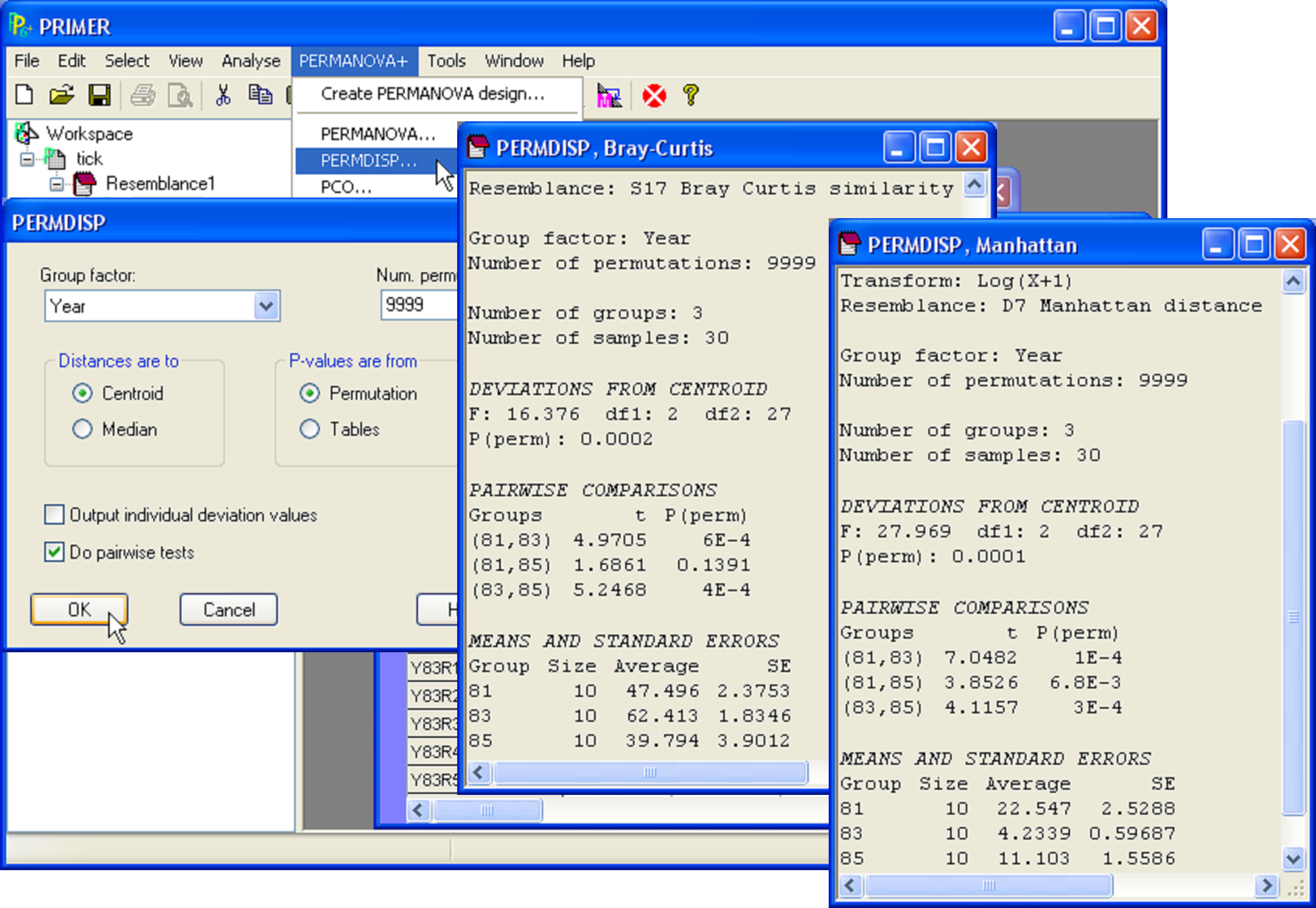
Fig. 2.6. PERMDISP for Tikus Island coral data using Bray-Curtis, and also using Manhattan distances on log(x+1)-transformed data.
One of the important reasons for the large dissimilarities among samples in 1983 was because the El Niño caused a massive coral bleaching event, and many of the corals died. Those that remained were very patchy, were generally not the same species in different transects and had small cover values. A quick scan of the data file reveals the large number of zeros recorded in 1983; none of the coral species achieved percentage cover values above 4%. The sparse data in 1983 therefore yielded many Bray-Curtis similarities of zero (dissimilarities of 100%) among samples55.
55 Clarke, Somerfield & Chapman (2006) have discussed the potentially erratic behaviour and lack of discrimination of the Bray-Curtis measure for sparse data such as these, proposing an adjustment which consists of adding a “dummy” species (present everywhere) into the dataset. They show that, for these coral data, the adjustment does have the effect of stabilising the dispersion across years and optimising the year-to-year separation.
2.8 Choice of measure
An extremely important point is that the test of dispersion is going to be critically affected by the transformation, standardisation and resemblance measure used as the basis of the analysis. It is pretty well appreciated by most practitioners that transforming the data has important effects on relative dispersions. Consider the fact that one of the common remedies to heterogeneity of variances in the analysis of univariate data is indeed to perform an appropriate transformation (e.g., Box & Cox (1964) ). Such a transformation is (usually) designed explicitly to make the data more normally distributed (less skewed), to remove intrinsic mean-variance relationships (if any), and to render the variances essentially homogeneous among groups. Although the consequences of the use of transformations on resulting inferences is rarely articulated explicitly ( McArdle & Anderson (2004) ), such an approach has merit and is widely used in univariate analyses. Thus, it is not at all difficult to understand that transformations will also affect relative dispersions in multivariate space.
Much less well appreciated is the extent to which the choice of resemblance measure can affect perceived patterns and results regarding relative dispersions among groups. For example, consider the analysis of the percentage cover data on corals from South Tikus Island. The Bray-Curtis measure is known to display erratic behaviour for sparse data such as these ( Clarke, Somerfield & Chapman (2006) ). We might consider an analysis of the same dataset using some other measure, such as a Euclidean or Manhattan distance on log(x+1)-transformed cover values. Such an approach could be considered reasonable on the grounds that the transformation will appropriately reduce the effects of large cover values, and a measure such as the Manhattan distance does not exclude joint absence information. In the present context, the joint absences of coral species (having been killed by bleaching) might indeed be considered to indicate similarity between samples. An MDS of the samples on the basis of the Manhattan measure on log(x+1)-transformed values shows a dramatically different pattern to what was shown using the Bray-Curtis measure (cf. Fig. 2.7 with Fig. 2.5). The points corresponding to samples from 1983 form a very tight cluster, samples from 1985 are a bit more dispersed, and the dispersion among samples from 1981 are much more dispersed (Fig. 2.7). The results of the PERMDISP analysis indicate that these differences in relative within-group dispersions among the groups (1981 > 1985 > 1983) are all highly statistically significant (see Fig. 2.6 above).
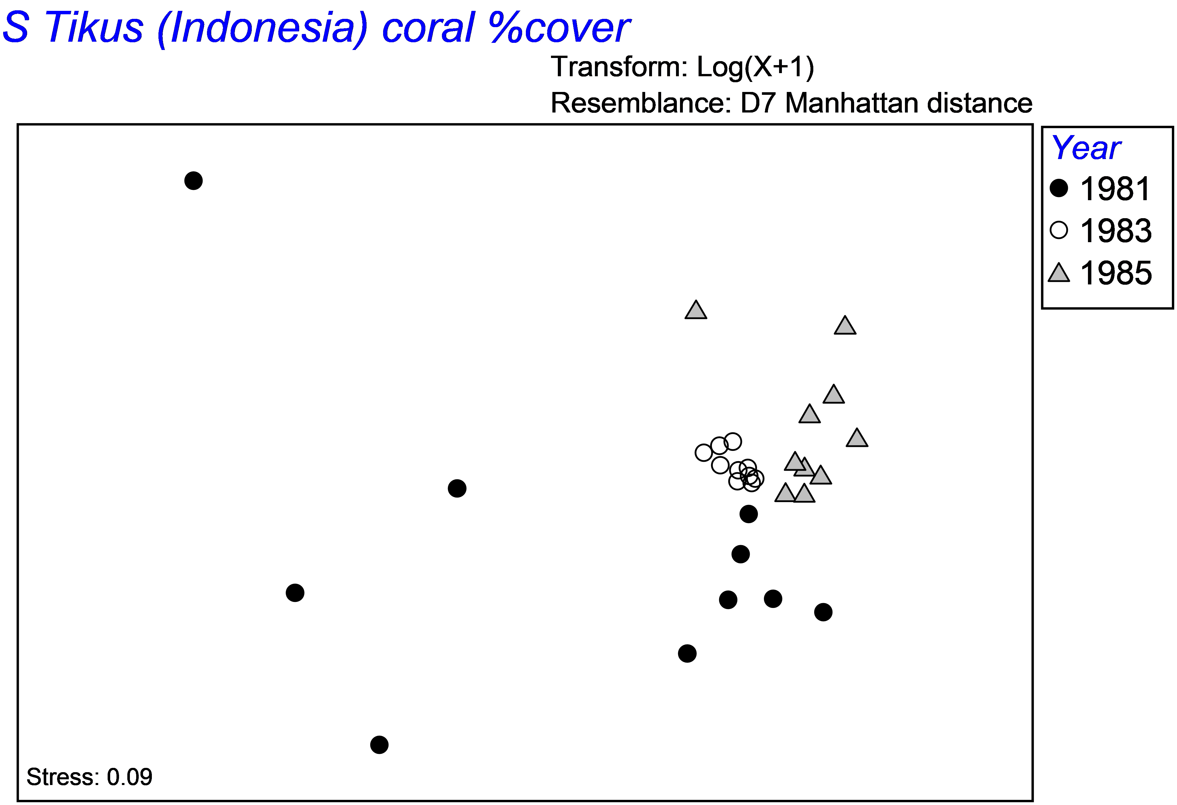
Fig. 2.7. MDS of coral assemblages from South Tikus Island in each of three years on the basis of Manhattan distances of log(x+1)-transformed percentage cover.
What we mean when we say “heterogeneity in multivariate dispersions” therefore must be qualified by reference to the particular resemblance measure we have chosen to use. Clearly, in the present case, the inclusion or exclusion of joint absence information can dramatically alter the results. In this particular example, the effects of transformations were actually quite modest by comparison56. Of course, the nature of the patterns obtained in any particular case will depend, however, on the nature of the data. In some cases, the transformation chosen will have dramatic effects.
There are many new areas to explore concerning the effects of different resemblance measures and transformations on relative within-group dispersions in different situations. The point is: be careful to define what is meant by “variability in assemblage structure” and realise that this is specific to the measure you have chosen to use and the nature of your particular data. Also, if you are intending to analyse the data using PERMANOVA as well, then of course it makes sense to choose the same transformation/standardisation/resemblance measure for the PERMDISP routine as were used for the PERMANOVA in order to obtain reasonable joint interpretations and inferences.
In addition, as PERMANOVA uses common measures of variability in the construction of F-ratios for tests, homogeneity is definitely implicit in the analysis of a resemblance matrix using PERMANOVA. Thus, after calculating a resemblance matrix which captures the desired ecological/community properties of the data, analysis by PERMDISP and visual assessment in ordination plots will highlight potential heterogeneities that could lead to a suitable degree of caution in the interpretation of results from a PERMANOVA model of the variation. This is not to say that a non-significant result using PERMDISP is an absolute requirement before using PERMANOVA; it is expected that PERMDISP will be powerful enough to detect small differences in dispersion that may not affect PERMANOVA adversely. However, the closer one can get to stabilising the relative dispersions among groups (or among cells in higher-way designs, etc.), the more valid and clear will be the interpretations from a PERMANOVA analysis.
56 Results obtained using Bray-Curtis on log(x+1)-transformed data are similar to what is obtained in Fig. 2.5 and results obtained using Manhattan on untransformed data are similar to what is obtained in Fig. 2.7 (try it)!
2.9 Dispersion as beta diversity (Norwegian macrofauna)
When used on species composition (presence/absence) data in conjunction with certain resemblance measures, the test for homogeneity of multivariate dispersions is directly interpretable as a test for similarity in beta diversity among groups ( Anderson, Ellingsen & McArdle (2006) ). Whittaker ( Whittaker (1960) , Whittaker (1972) ) defined beta diversity as the degree to which a set of observations in a given geographical area vary in the identities of species they contain. More specifically, he proposed a measure of beta diversity as the proportion by which a given area is richer than the average of the samples within it. Although there may be many ways to define beta diversity (e.g., Vellend (2001) , Magurran (2004) ), Anderson, Ellingsen & McArdle (2006) considered that beta diversity can be broadly defined as the variability in species composition among sampling units for a given area at a given spatial scale. Whittaker’s measure (as a proportion) only provides a single value per area (or group), so cannot be used to test for differences among groups in beta diversity57. However, PERMDISP on the basis of ecological measures of compositional dissimilarity (e.g., Jaccard or Sørensen, which is just Bray-Curtis on presence/absence data) can be used for such a test. Note that the definition of beta diversity is focused on variability in composition. Thus, multivariate dispersion on the basis of any resemblance measure that includes relative abundance information as well will not necessarily provide a measure of beta diversity, per se.58
Ellingsen & Gray (2002) studied beta diversity and its relationship with environmental heterogeneity in benthic marine systems over large spatial scales in the North Sea. Samples of soft-sediment macrobenthic organisms were obtained from N = 101 sites occurring in five large areas along a transect of 15 degrees of latitude (Fig. 2.8). A total of p = 809 taxa were recorded overall, and samples consisted of abundances pooled across five benthic grabs obtained at each site. The upper 5 cm of one additional grab was also sampled to measure environmental variables at each site. Of interest was to measure beta diversity (the degree of compositional heterogeneity) for each of these five areas and to compare this with variation in the environmental variables. The biological data are provided in the file norbio.pri in the ‘NorMac’ folder in the ‘Examples add-on’ directory.
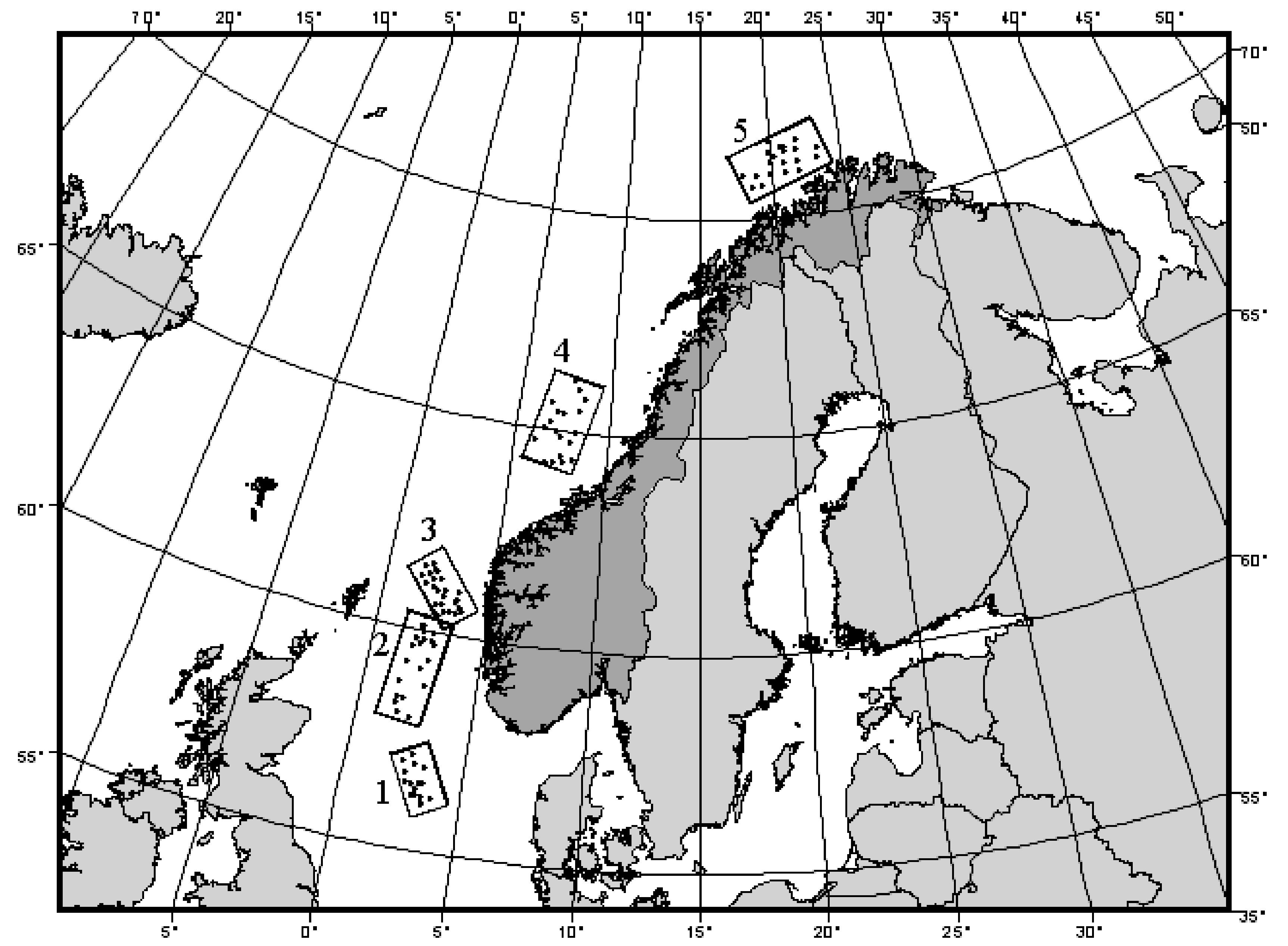
Fig. 2.8. Map showing locations of samples of macrobenthic fauna taken from each of 5 areas in the North Sea (after Ellingsen & Gray (2002) ).
An MDS plot on the basis of the Jaccard measure shows patterns of differences in assemblage composition among the five areas (Fig. 2.9). The Jaccard measure is directly interpretable as the percentage of unshared species. It uses only presence/absence information and measures of multivariate dispersion based on this measure are indeed interpretable as measures of beta diversity. Perhaps the most striking thing emerging from the plot is the quite large spread of sample points corresponding to area 3 and the quite tight cluster of points corresponding to area 1 compared to the other areas. The test for homogeneity reveals very strong differences among the five groups and, more particularly, identifies group 1 and group 3 as being significantly different from one another and from the other three groups (2, 4 and 5) in terms of their variability in species composition59 (Fig. 2.9). The average Jaccard distance-to-centroid is about 36% for group 1, but is much larger (more than 56%) for group 3. This pattern of heterogeneity was mirrored by similar patterns of variability in the environmental variables for the three areas (see Ellingsen & Gray (2002) and Anderson, Ellingsen & McArdle (2006) for more details). One possible explanation for the relatively large biological and environmental variation in area 3 is that this may be an area of rapid transition from the southern to the northern climes.
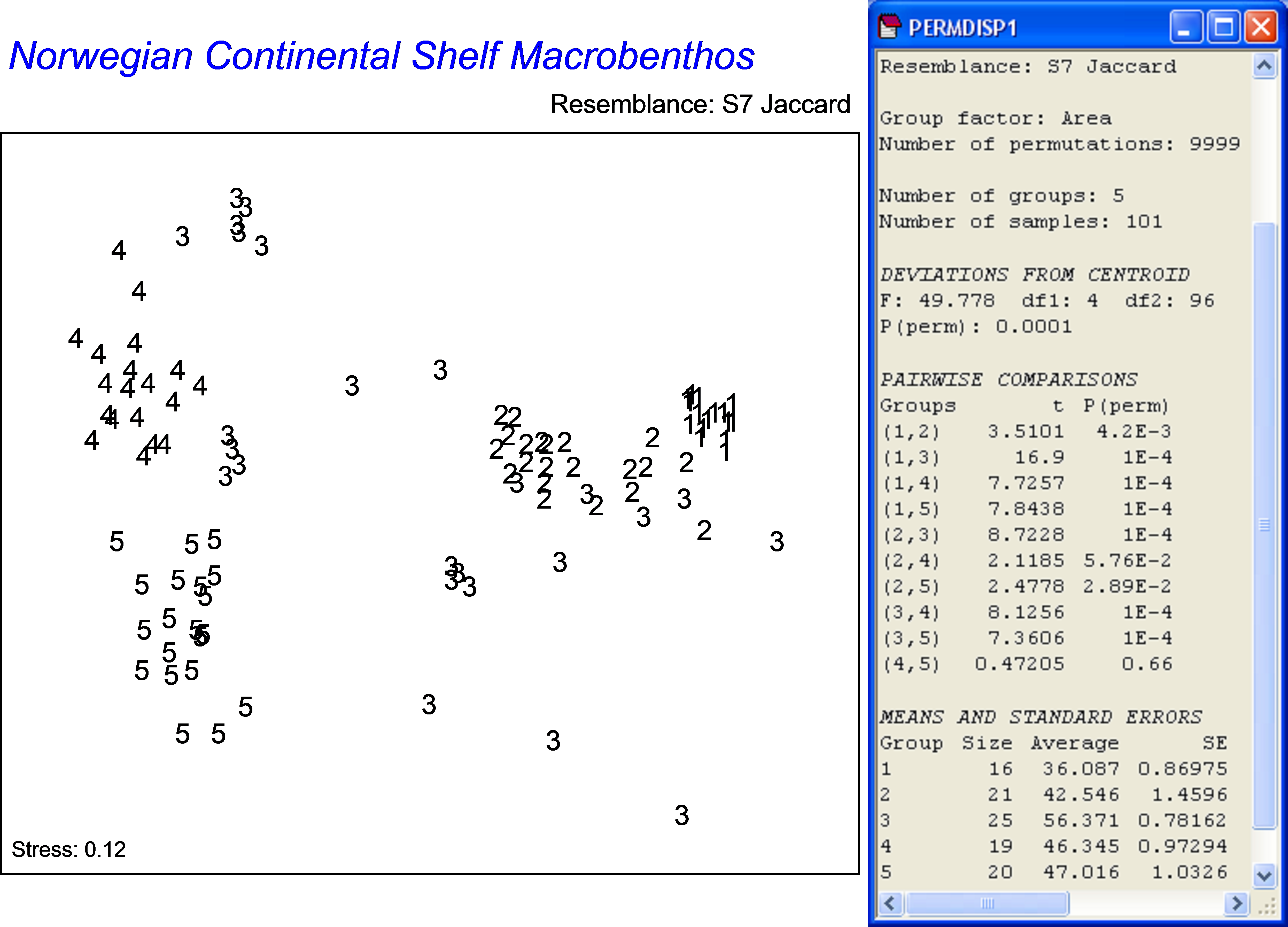
Fig. 2.9. MDS of Norwegian macrofauna from 5 areas (labelled 1-5 as on the map in Fig. 2.8) based on the Jaccard measure and the results of PERMDISP, alongside, comparing beta diversity among the 5 areas.
57 See Kiflawi & Spencer (2004) , however, who have shown how expressing beta diversities in terms of an odds ratio does allow confidence intervals to be constructed.
58 If we allow dispersion based on any resemblance measure to be considered “beta diversity”, then beta diversity simply becomes a non-concept (sensu Hurlbert (1971) ). For example, compare Figures 2.5 and 2.7; surely we cannot claim that both of these describe relative patterns in beta diversity for the same dataset!
59 Note that in PERMDISP, as in PERMANOVA, the pairwise tests are not corrected for multiple comparisons. See the section on Pairwise comparisons in chapter 1 on PERMANOVA for more details
2.10 Small sample sizes
There is one necessary restriction on the use of PERMDISP, which is that the number of replicate samples per group must exceed n = 2. The reason is that, if there are only two replicates, then, by definition, the distance to the centroid for those two samples must be equal to one another. Consider a single variable and a group with two samples having values of 4 and 6. The centroid (average) in Euclidean space for this group is therefore 5. The distance from sample 1 to the centroid is 1 and the distance from sample 2 to the centroid is also 1. These two values of z are necessarily equal to one another. This will also be the case for other groups having only 2 replicate samples, so the within-group variance of the z’s when n = 2 for all groups will be equal to zero. If the within-group variance is equal to zero, then the F statistic will be infinite, so the test loses all meaning. Clearly, the test is also meaningless for a group with n = 1, which will have only a single z value of zero. Thus, if the sample size for any of the groups is n ≤ 2, then the PERMDISP routine will issue a warning accordingly. Although test results are meaningless in such cases, the individual deviations (the z’s) can nevertheless still be examined and compared in their value across the different groups, if desired. More generally, the issue here is the degree of correlation among values of z, which increases the smaller the sample size. Levene (1960) showed the degree of correlation is of order n-2 which, he suggested, will probably not have a serious effect on the distribution of the F statistic. We suggest that formal tests using PERMDISP having within-group sample sizes less than n = 10 should be viewed with some caution and those having sample sizes less than n = 5 should probably be avoided, though (as elsewhere) further simulation studies for realistic multivariate cases would be helpful in refining such rules-of-thumb.
2.11 Dispersion in nested designs (Okura macrofauna)
In many situations, the experimental design is not as simple as a one-way analysis among groups. For more complex designs, several tests of dispersion may be possible and relevant at a number of different levels. The sort of tests that will be logical to do in any given situation will depend on the design and the nature of existing location effects (if any) that were detected by PERMANOVA. This is particularly the case when factors can interact with one another (see the section on crossed designs). First, however, we shall consider relevant tests of dispersion that might be of interest in the case of a nested experimental design. For simplicity, we shall limit our discussion here to the two-factor nested design, although the essential principles discussed will of course apply to situations where there are greater numbers of factors in a nested hierarchy.
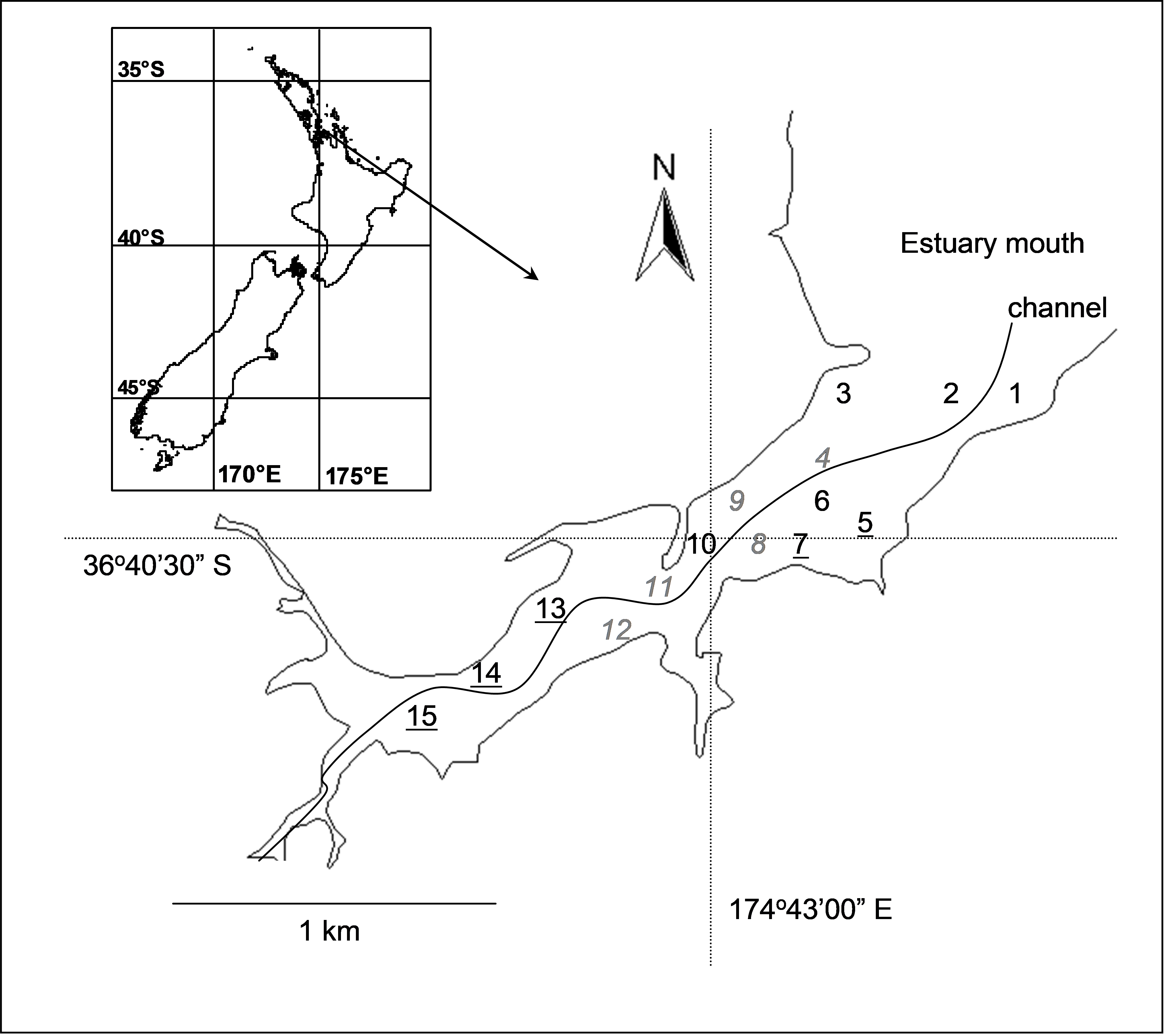 Fig. 2.10. Okura estuary, with the 15 sites for sampling of benthic fauna labeled: high depositional sites are underlined, medium depositional sites are in italics and low depositional sites are in normal font.
Consider the experimental design described by Anderson, Ford, Feary et al. (2004) investigating the potential effects of different depositional environments on benthic intertidal fauna of the Okura estuary in New Zealand. The hydrology and sediment dynamics of the estuary had been previously modeled ( Cooper, Green, Norkko et al. (1999) , Green & Oldman (1999) ), and areas corresponding to high, medium or low probability of sediment deposition were identified. There were n = 6 sediment cores (13 cm in diameter × 15 cm deep) obtained from random positions within each of 15 sites along the estuary, with 5 sites from each of the high, medium and low depositional types of environments (Fig. 2.10). Sampling was repeated 6 times (twice in each of three seasons in 2001-2002), but we shall focus for simplicity on the following spatially nested design for the first time of sampling only:
-
Factor A: Deposition (fixed with a = 3 levels, high (H), medium (M) or low (L)).
-
Factor B: Site (random with b = 5 levels, nested in Deposition).
The design was balanced, with n = 6 replicate cores per site for a total of N = a × b × n = 90 samples obtained at each time. The data (counts of p = 73 taxa) are located in the file okura.pri in the ‘Okura’ folder of the ‘Examples add-on’ directory. We shall follow Anderson, Ford, Feary et al. (2004) and perform the analysis on the basis of the Bray-Curtis measure on log(x+1)-transformed abundances. An MDS plot of the data from time 1 only (Fig. 2.11) revealed a fairly clear pattern to suggest that assemblages from different depositional environments were distinguishable from one another, especially those from sites having relatively high probabilities of deposition.
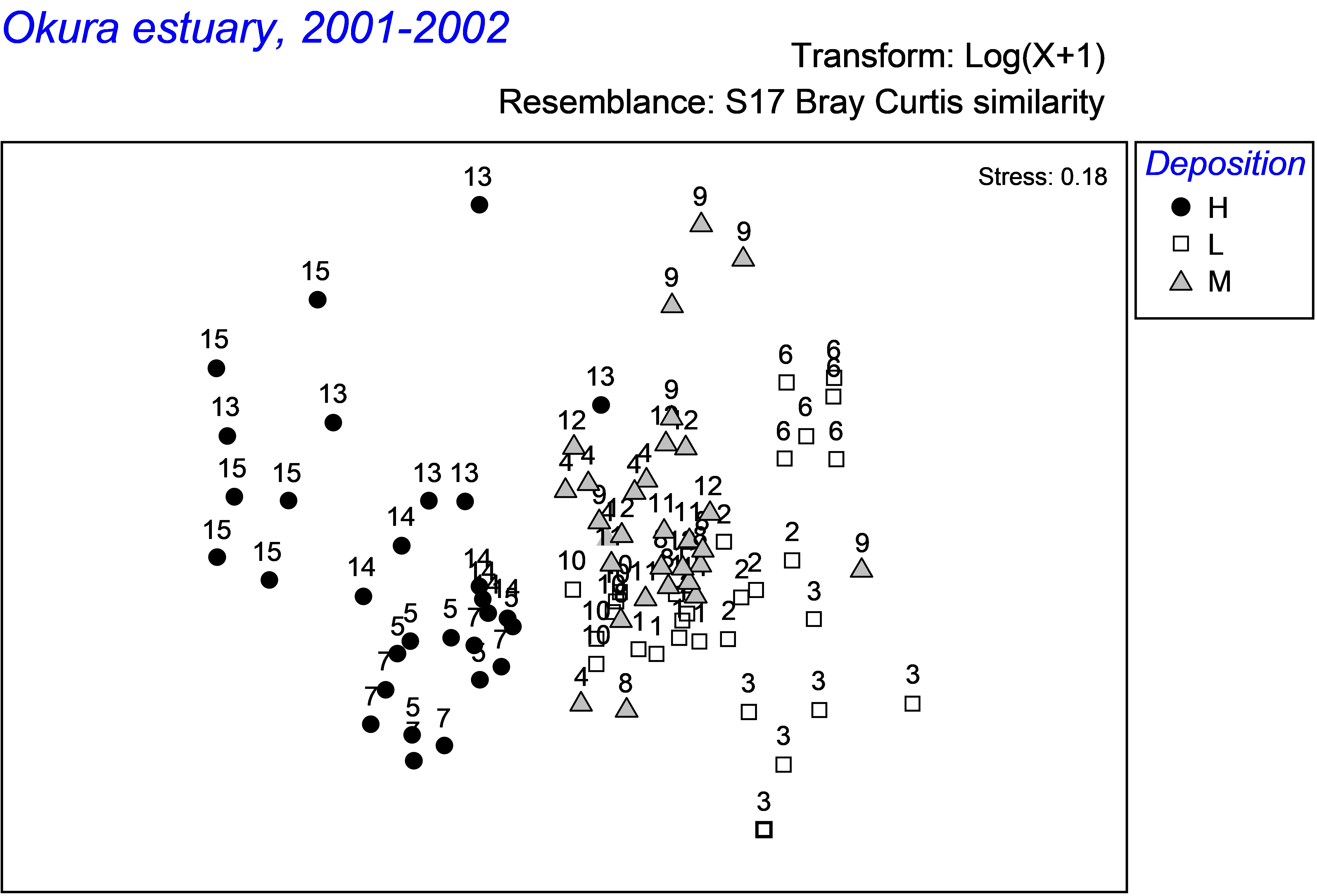 Fig. 2.11. MDS of assemblages of intertidal soft-sediment infauna from Okura estuary at each of 15 sites (numbered as in Fig. 2.10) having high (H), medium (M) or low (L) probabilities of sediment deposition.
For a design such as this, there are two levels at which we may wish to think about relative dispersions. First, are the multivariate dispersions among the 6 cores within a site different among sites? Second, are the multivariate dispersions among the 5 site centroids different among the three different depositional environments? Another (third) possibility might be to compare the dispersions of the 5 × 6 = 30 cores across the three depositional environments. However, such a test would only really be logical if there were no differences in location among sites (i.e. no significant ‘Site’ effects in the PERMANOVA).
First, consider the variability among cores within each site. For these particular data, the 15 sites are labeled 1-15 according to their position in the estuary (Fig. 2.10). Thus, to compare dispersions of assemblages in cores across sites, we simply run PERMDISP on the factor ‘Site’ for the full resemblance matrix. Note that these a × b = 15 cells correspond to the lowest-level cells in the design. If the sites had been labeled 1-5, that is, if the sites had been given the same labels within each of the depositional environments (even though they are different actual sites, being nested), then we would have to first create a new factor corresponding to the fifteen cells (all combinations of factors A and B) by choosing Edit > Factors > Combine.
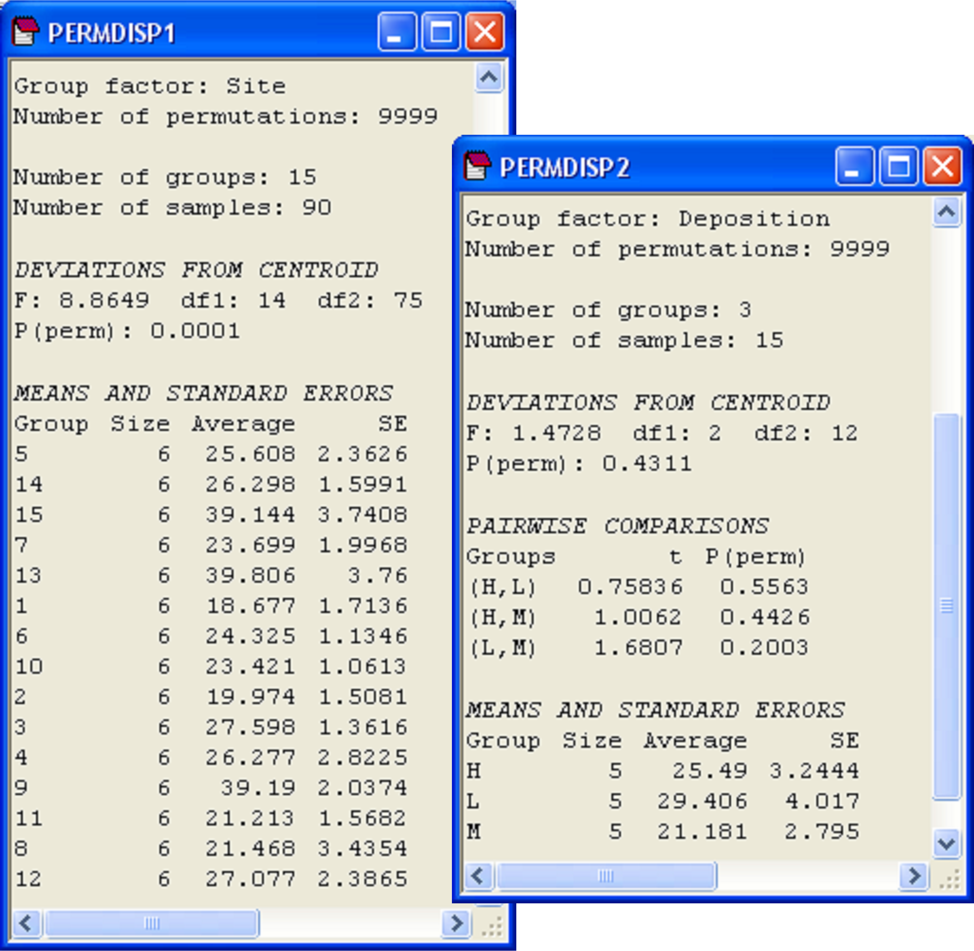 Fig. 2.12. PERMDISP analyses for a nested design done at two levels: comparing variability among cores across sites (left) and comparing variability among sites across depositional environments (right).
This first PERMDISP analysis reveals that the dispersion among cores varies significantly from site to site (Fig. 2.12, F = 8.86, P < 0.001). As ‘Site’ is a random factor, we are not especially interested in performing pairwise comparisons here, so these have not been done. There is heterogeneity in dispersions among cells and examining the output reveals that the average distance-to-centroid in Bray-Curtis space within a site generally varies from about 18 to 27%. Three of the sites, however, have an average distance-to-centroid of nearly 40% (Fig. 2.12).
Next, we shall consider the second question posed above: are there differences in the dispersions of the 5 site centroids for different depositional environments? Before proceeding, we first need to obtain a distance matrix among the site centroids. Recall, however, that the centroids in Bray-Curtis (or some other non-Euclidean space) are not the same as the arithmetic centroids calculated on the original variables. Thus, unfortunately, we cannot calculate the site centroids by going back to the raw data and just calculating site averages for the original variables. Instead, we shall use a new tool available as part of the PERMANOVA+ add-on, which calculates a resemblance matrix among centroids for groups identified by a factor in the space of the chosen resemblance measure. To do this for the present example, click on the resemblance matrix and then choose PERMANOVA+ > Distances among centroids… > Grouping factor: Site, then click ‘OK’. The resulting resemblance matrix contains the correct Bray-Curtis dissimilarities among the site centroids, which have been calculated using PCO axes (see the section Generalisation to dissimilarities). Just to re-iterate, these centroids are not calculated on the original data, they are calculated on PCO axes obtained from the resemblance matrix, in order to preserve the resemblance measure chosen as the basis of the analysis.
To visualise the relative positions of centroids in multivariate space, choose Analyse > MDS from this resemblance matrix among centroids. Conveniently, PRIMER has retained all of the factors and labels associated with these points, so we can easily place appropriate labels and symbols onto the centroids in the plot. The dispersions of the site centroids appear to be roughly similar for the three depositional environments (H, M and L, Fig. 2.13), and indeed the test for homogeneity of dispersions revealed no significant differences among these three groups (Fig. 2.12, F = 1.47, P = 0.43). Note that ‘Deposition’ is a fixed factor and so we would indeed have been interested in the pair-wise comparisons among the three groups (had there been a significant F-ratio). This is why the option $\checkmark$Do pairwise tests was chosen; these results are also shown in the output (Fig. 2.12).
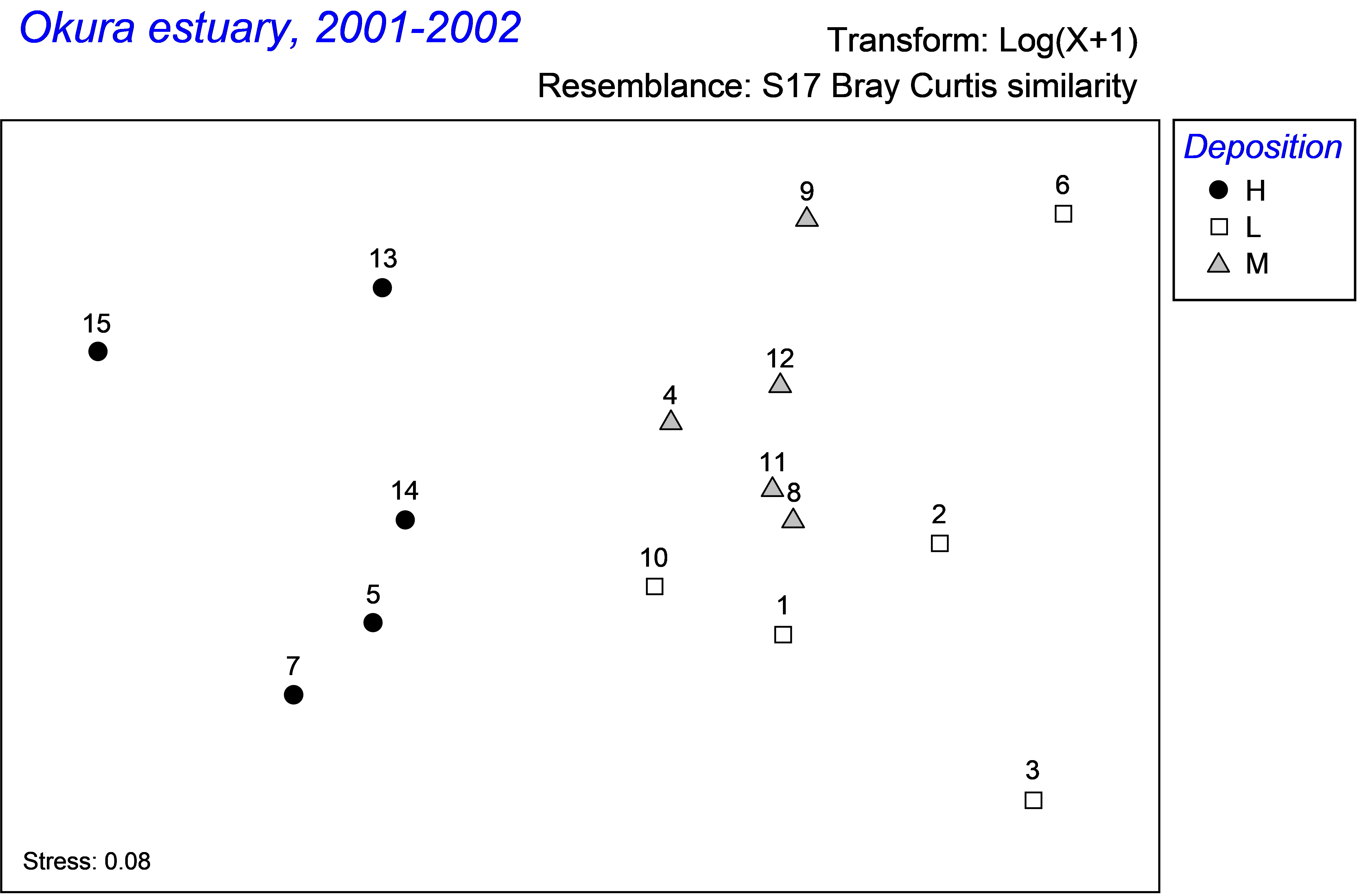 Fig. 2.13. MDS of site centroids for the Okura data obtained from PCO axes on the basis of the Bray-Curtis resemblance measure of log(x+1)-transformed abundances.
Finally, we may consider the third question above: are there differences in dispersions among cores (ignoring sites) for the three depositional environments? Such a question only makes sense if sites have no effects. However, the results of the two-factor PERMANOVA for this experimental design reveals that ‘Site’ effects are highly statistically significant (pseudo-F = 5.49, P < 0.001, Fig. 2.14). Therefore, there is no logical reason to consider the multivariate dispersion of cores in a manner that ignores sites. As an added note of interest, the PERMANOVA test of the factor ‘Deposition’ in the two-factor nested design yields the same results as a one-way PERMANOVA for ‘Deposition’ using the resemblance matrix among site centroids (pseudo-F = 4.56 with 2 and 12 df, P < 0.001, Fig. 2.14). This clarifies how the nested model effectively treats the levels of the nested term (in this case, ‘sites’) as replicates for the analysis of the upper-level factor. Note that this equivalence would not hold if the centroids had been calculated as averages from the raw (or even the transformed) original data, which further emphasises that the centroids obtained using PCOs are indeed the correct ones for the analysis.
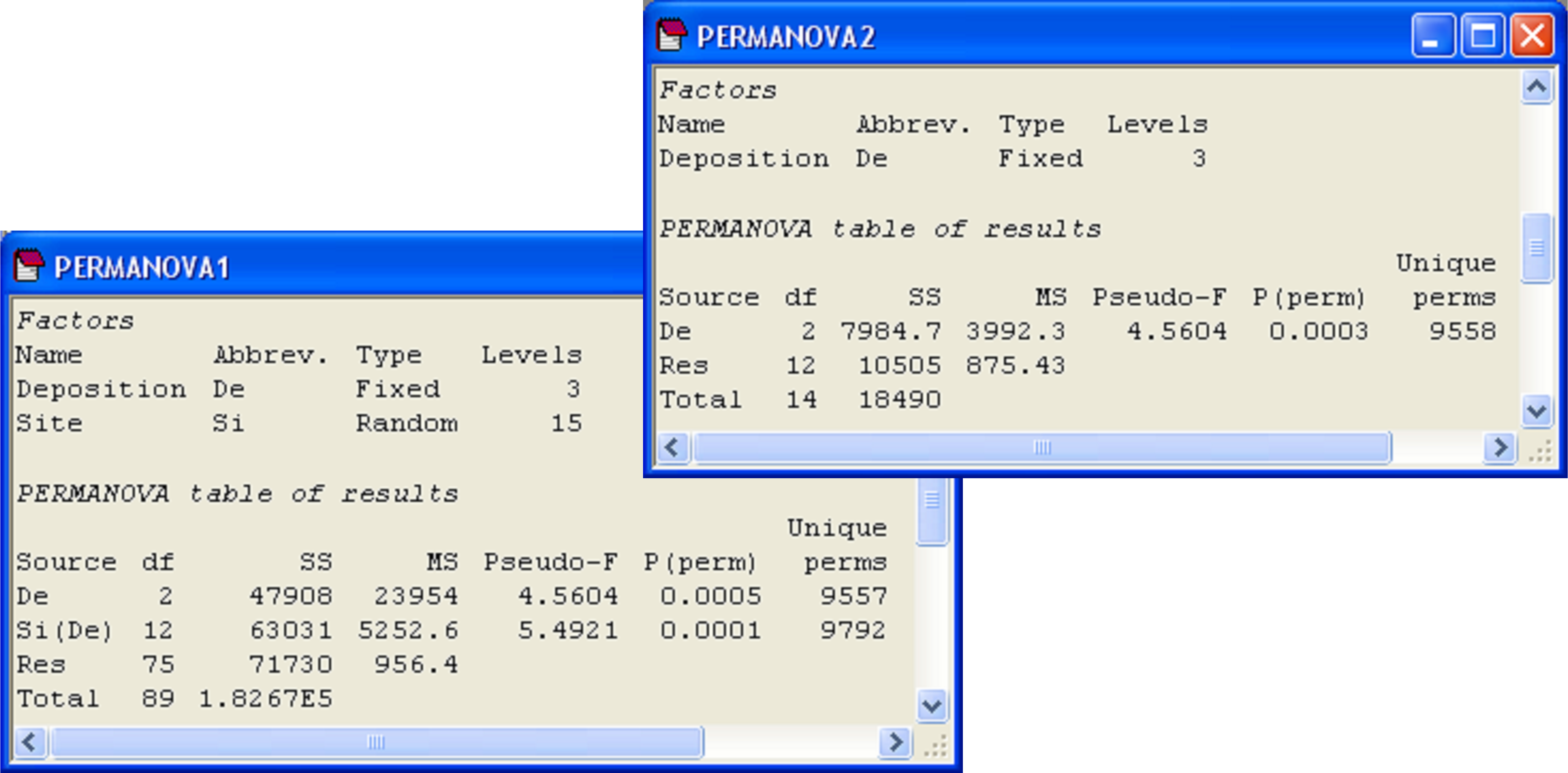 Fig. 2.14. PERMANOVA of the Okura data from time 1 according to the two-factor nested design and the test for depositional effects alone in a one-factor design on the basis of resemblances among site centroids.
2.12 Dispersion in crossed designs (Cryptic fish)
When two factors are crossed with one another, there may be several possible hypotheses concerning relative dispersions among groups. An important aspect of analysing multi-factorial designs is to keep straight when you are focusing on dispersion effects and when you are focusing on location effects. Running PERMANOVA and PERMDISP in tandem, driven by carefully articulated hypotheses, provides a useful general approach.
Here we shall consider a study to investigate effects of marine reserve status and habitat on cryptic fish assemblages in northeast New Zealand, as described by Willis & Anderson (2003) . Although marine reserves in this region afford protection for larger exploited fish species (such as snapper, Pagrus auratus, which occur in greater relative abundances and sizes inside reserves, see Willis, Millar & Babcock (2003) ), relatively little is known regarding the potential flow-on effects (either positive or negative) on many of the other components of these ecosystems (but do see Shears & Babcock (2002) , Shears & Babcock (2003) regarding habitat-scale effects). For example, do assemblages of smaller and/or more cryptic fish (such as triplefins and gobies) change with increased densities of predators inside versus outside marine reserves? Is this effect (if any) modified in kelp forest habitat as opposed to urchin-grazed ‘barrens’ habitat? The two factors in the design were:
-
Factor A: Status (fixed with a = 2 levels, reserve (R) or non-reserve (N) sites).
-
Factor B: Habitat (fixed with b = 2 levels, kelp forest (k) or urchin-grazed rock flats (r), crossed with Status).
There were n = 6 replicate 9 m$^2$ plots surveyed within each of the a × b = 4 combinations of levels of the above two factors, yielding counts of abundances for p = 33 species. These data are located in the file cryptic.pri in the ‘Cryptic’ folder of the ‘Examples add-on’ directory. An MDS on the basis of the Bray-Curtis measure on square-root transformed abundances does not show very clear effects of either of these factors (Fig. 2.15). Formal tests are necessary to clarify whether any significant effects of either factor (or their interaction) are detectable in the higher-dimensional multivariate space.
 Fig. 2.15. MDS of cryptic fish assemblages at reserve (R) or non-reserve (N) sites in either kelp forest or urchin-grazed rock flat habitats.
First, we shall run a PERMANOVA on the two-factor design, bearing in mind that the test is specifically designed to detect location effects, but dispersion effects (if any) might also be detected by this test. Results indicate that the two factors do not interact (P > 0.70), but there are significant independent effects of ‘Status’ and ‘Habitat’ (P < 0.01 in each case, Fig. 2.16).
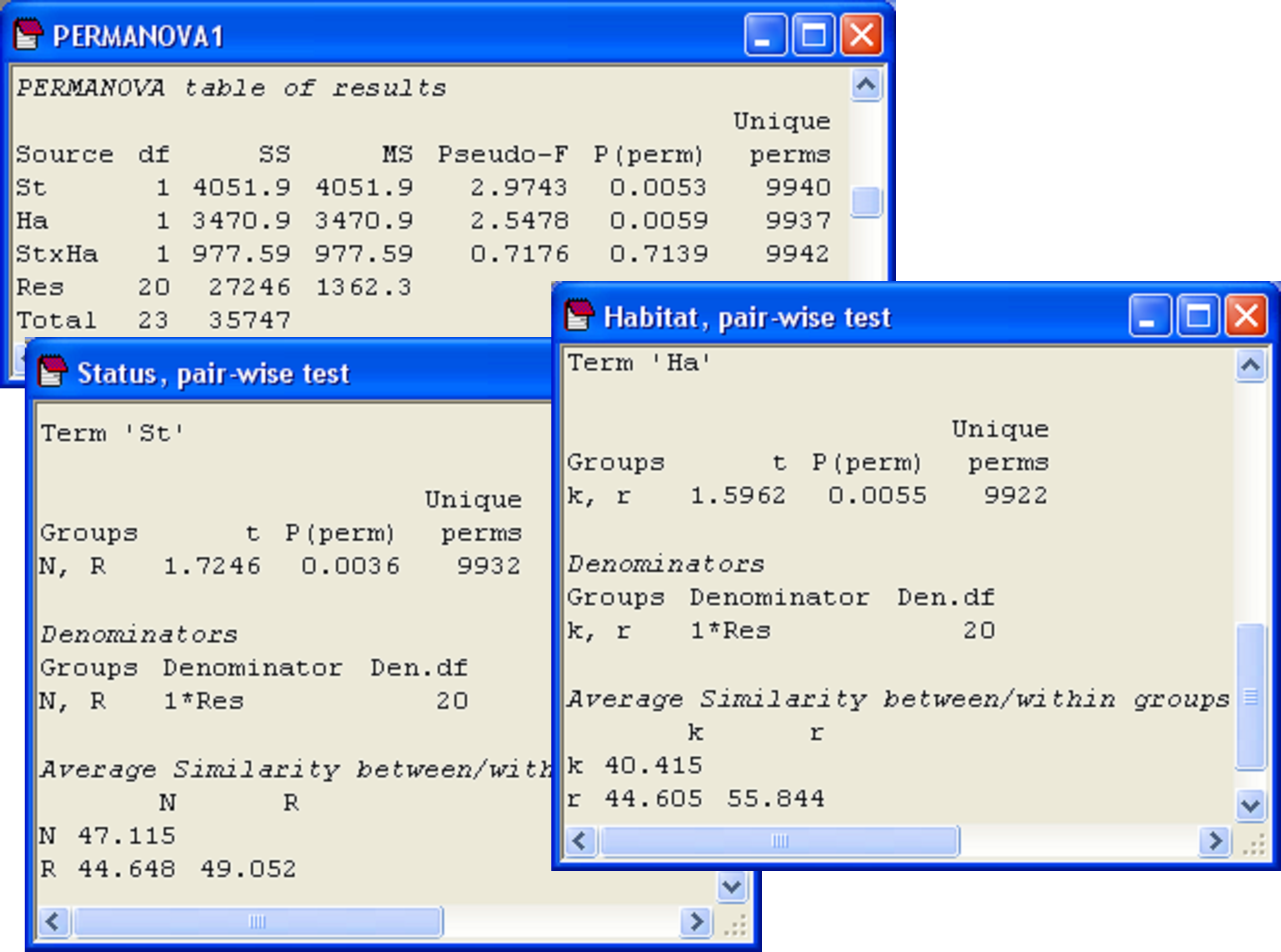 Fig. 2.16. PERMANOVA for the two-way analysis of cryptic fish, along with pair-wise comparisons for each of the main effects.
Although there are only two levels of each of the factors (so the tests in the main PERMANOVA analysis are enough to indicate the significant difference between the two levels, in each case), pair-wise comparisons done on each factor will give us a little more information regarding the average similarity between and within the different groups (Fig. 2.16). The average within-group similarities are comparable for ‘N’ and ‘R’, but the average within-group similarity in the kelp forest habitat (‘k’, 40.4%) is much smaller than that in the rock flat habitat (‘r’, 55.8%). The former is even smaller than the average similarity between kelp and rock-flat habitats (44.6%)! The pattern in the MDS plot (Fig. 2.15) also indicates greater dispersion of points for ‘k’ (squares) than for ‘r’ (downward triangles). These observations provide signals to suggest (but do not prove) that the significant effect of habitat might be driven somewhat by differences in dispersions. Of course, we can investigate this idea formally using PERMDISP.
First, although there is no significant interaction detected by PERMANOVA, it is still possible that the individual cells may differ in their relative dispersions. This can be tested by combining the two factors to make a single factor with a × b = 4 levels and then running PERMDISP to compare these within-cell dispersions. Choose Edit > Factors > Combine and then ‘Include’ both factors in the ‘Ordered selection’ dialog box (Fig. 2.17). Next choose PERMANOVA+ > PERMDISP > (Group factor: StatusHabitat) & (Distances are to •Centroids) & (P-values are from •Permutation) & (Num. permutations: 9999). For these data, the null hypothesis of equal dispersions among the four cells is retained (F = 2.0, P > 0.25, Fig. 2.17).
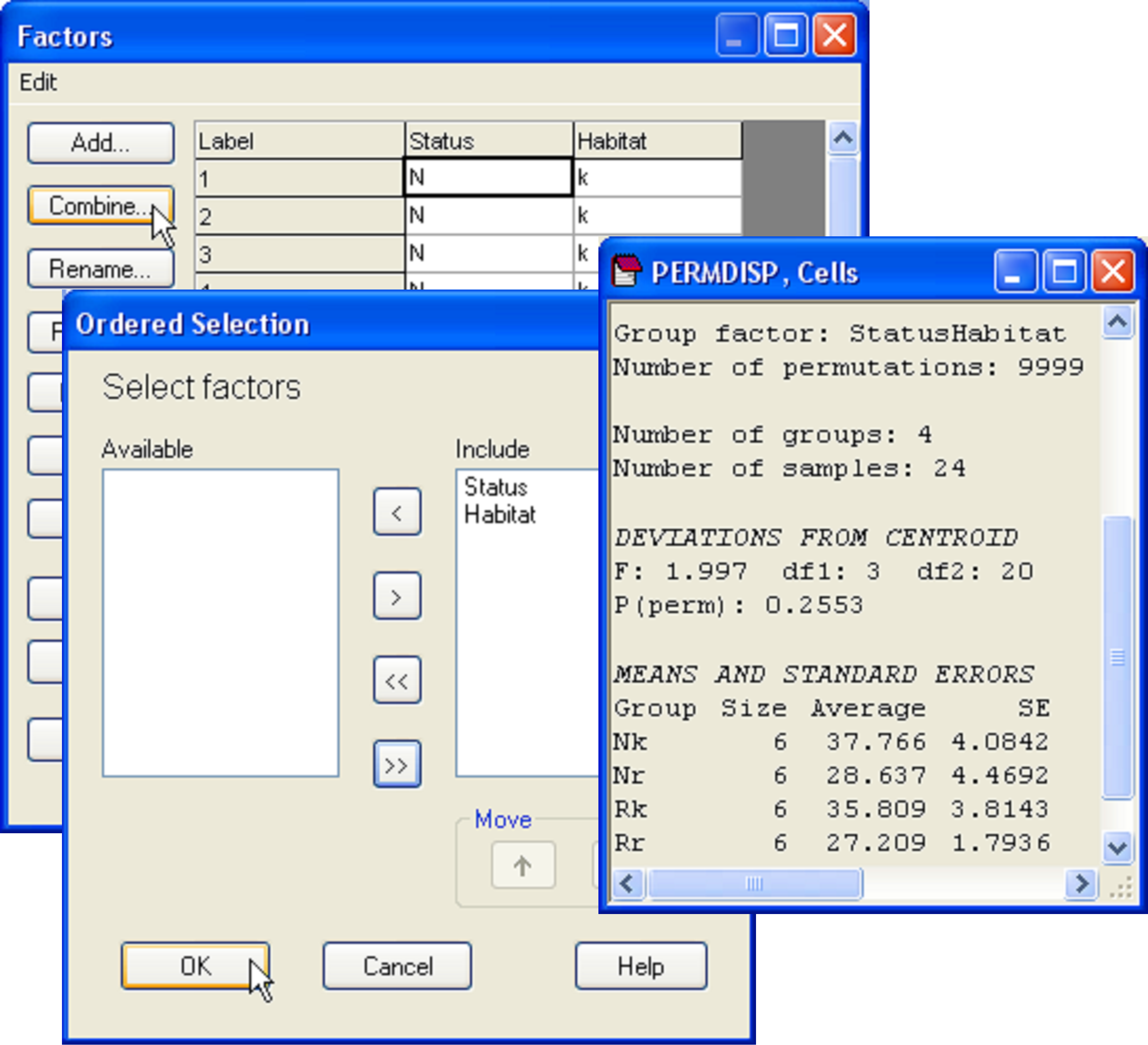 Fig. 2.17.
Menus used to generate a combined factor consisting of the 4 combinations of ‘Status’ and ‘Habitat’, and the results window from PERMDISP which formally compares dispersions among these four cells.
Fig. 2.17.
Menus used to generate a combined factor consisting of the 4 combinations of ‘Status’ and ‘Habitat’, and the results window from PERMDISP which formally compares dispersions among these four cells.
Next, to consider analyses of dispersions for main effects in a crossed design (such as this), it is important to consider what might be meaningful in light of the PERMANOVA results. When two (or more) factors are crossed with one another, it is easily possible to confuse a dispersion effect with an interaction effect. To illustrate this point, suppose I have a two-factor design, where there is a significant interaction such as that shown in Fig. 2.18. More specifically, suppose there is no effect of factor A in level 1 of factor B (grey/filled symbols), but there is a significant effect of factor A in level 2 of factor B (white/open symbols). A test for equality of dispersions among the levels of factor B that ignored A would clearly find a significant difference between the two levels of factor B (with white symbols obviously being more dispersed than grey symbols). However, this is not really caused by dispersion differences per se, but rather is due to the fact that factor A interacts with factor B. Therefore, before performing tests of dispersion for main effects in crossed designs, the potential for interactions to confound interpretations of the results should be examined. This is generally achieved by first testing and investigating the nature of any significant interaction terms using PERMANOVA, and also by examining patterns in ordination plots.
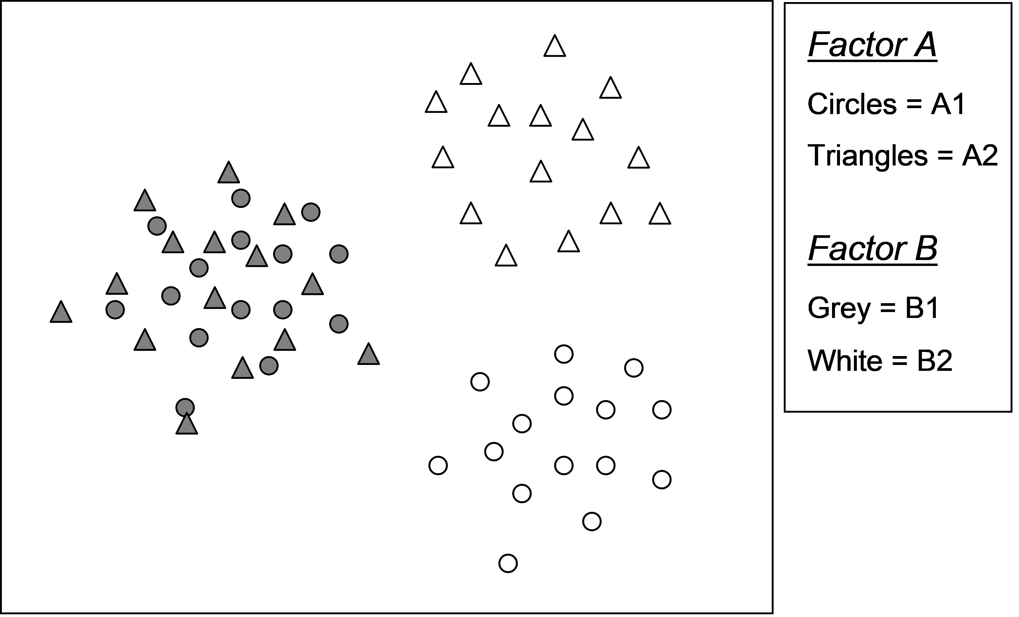
Fig. 2.18. Schematic diagram in two dimensions of an interaction between two factors that can result in misinterpretation of tests of dispersion for main effects.
We have seen, for the cryptic fish data, that no interaction was detected between ‘Status’ and ‘Habitat’ (Fig. 2.16), so we can perform the test of homogeneity of dispersions for each of the main effects separately (ignoring the other factor) using PERMDISP. These reveal no significant differences in dispersion for the ‘Status’ factor (F = 0.06, P > 0.82), but significant differences in dispersion for the ‘Habitat’ factor, with greater variability in the fish assemblages observed in kelp forests compared to the urchin-barrens rock flat habitat (F = 7.8, P < 0.05, Fig. 2.19)60.
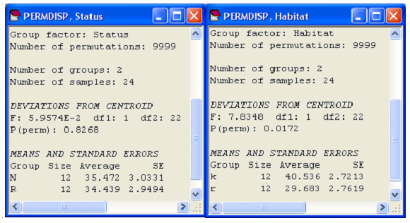
Fig. 2.19. Results of PERMDISP on each of the main effects from the two-factor study of cryptic fish.
Note that the significant effect of the marine reserve ‘Status’ detected by the PERMANOVA is therefore now interpretable to be purely (in essence) a location effect, as the test for homogeneity of dispersions for this factor was not significant. However, the effect of ‘Habitat’ appears to be primarily (although perhaps not entirely) driven by differences in dispersion, with greater variability in the structure of cryptic fish assemblages observed in kelp forest habitats compared to rock flat habitats. If there is a location effect (i.e. a shift in multivariate space) due to habitat in addition to the dispersion effect detected (which of course is possible), then this should be discernible in MDS plots (preferably carried out separately for each reserve status in 3-d, when the stress will drop to lower values than in Fig. 2.15).
60 A word of warning: PERMDISP analyses and measures of dispersion for main effects like this will include the location shifts (if any) of other main effects. Although this won’t necessarily confound the analysis if the factors do not interact, it can nevertheless compromise power. Ideally, we would like to remove location effects of all potential factors before proceeding with the test. This is not implemented in the current version of PERMDISP, but there is clearly scope for further development here.
2.13 Concluding remarks
PERMDISP is designed to test the null hypothesis of no differences in dispersions among a priori groups. Although this may be the only goal in some cases, PERMDISP can also provide a useful companion test to PERMANOVA in order to clarify the nature of multivariate effects on the basis of a chosen resemblance measure.
Table 2.1 provides a synopsis of the logical inferences arising from the outcomes of PERMDISP and PERMANOVA for the one-way (single-factor) case. Three of the four scenarios yield a clear inferential outcome; the fourth leaves some uncertainty for interpretation. Namely, if both PERMDISP and PERMANOVA tests are significant, we will know that dispersion effects occur, but we may not necessarily know if location effects are also present. Examining ordination plots and the relative sizes of within and between-group resemblances will be important here, but it is undoubtedly true that there is scope for further work on the implications of a significant outcome for the PERMDISP test on the structure and interpretation of the associated PERMANOVA tests. Finally, in more complex designs with crossed or nested factors, several different PERMDISP analyses may be needed (e.g., at different levels in the design) in order to clarify dispersion effects, if any.
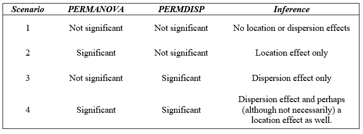
Table 2.1. Outcomes and potential inferences to be drawn from joint analyses done using PERMANOVA and PERMDISP for the one-way case.