Chapter 4: Distance-based linear models (DISTLM) and distance-based redundancy analysis (dbRDA)
Key references Method: Legendre & Anderson (1999), McArdle & Anderson (2001) Permutation methods: Freedman & Lane (1983), Anderson & Legendre (1999), Anderson & Robinson (2001), Anderson (2001b)
- 4.1 General description
- 4.2 Rationale
- 4.3 Partitioning
- 4.4 Simple linear regression (Clyde macrofauna)
- 4.5 Conditional tests
- 4.6 (Holdfast invertebrates)
- 4.7 Assumptions & diagnostics
- 4.8 Building models
- 4.9 Cautionary notes
- 4.10 (Ekofisk macrofauna)
- 4.11 Visualising models: dbRDA
- 4.12 Vector overlays in dbRDA
- 4.13 dbRDA plot for Ekofisk
- 4.14 Analysing variables in sets (Thau lagoon bacteria)
- 4.15 Categorical predictor variables (Oribatid mites)
- 4.16 DISTLM versus BEST/ BIOENV
4.1 General description
Key references
- Method: Legendre & Anderson (1999) , McArdle & Anderson (2001)
-
Permutation methods:
Freedman & Lane (1983)
,
Anderson & Legendre (1999)
,
Anderson & Robinson (2001)
,
Anderson (2001b)
DISTLM is a routine for analysing and modeling the relationship between a multivariate data cloud, as described by a resemblance matrix, and one or more predictor variables. For example, in ecology, the resemblance matrix commonly describes dissimilarities (or similarities) among a set of samples on the basis of multivariate species abundance data, and interest may lie in determining the relationship between this data cloud and one or more environmental variables that were measured for the same set of samples. The routine allows predictor variables to be fit individually or together in specified sets. P-values for testing the null hypothesis of no relationship (either for individual variables alone or conditional on other variables) are obtained using appropriate permutation methods. Not only does DISTLM provide quantitative measures and tests of the variation explained by one or more predictor variables, the new routine in PERMANOVA+ has a suite of new tools for building models and generating hypotheses. Parsimonious models can be built using a choice of model selection criteria and procedures. Coupled with preliminary diagnostics to assess multi-collinearity among predictor variables, several potentially relevant models can be explored. Finally, for a given model, the user may also visualise the fitted model in multi-dimensional space, using the dbRDA routine.
4.2 Rationale
Just as PERMANOVA does a partitioning of variation in a data cloud described by a resemblance matrix according to an ANOVA model, DISTLM does just such a partitioning, but according to a regression (or multiple regression) model. For an ANOVA design, the predictor variables are categorical (i.e., levels of factors), whereas in a regression model, the predictor variables are (generally) quantitative and continuous. ANOVA is simply a specific kind of linear model, so DISTLM can therefore also be used to analyse models that contain a mixture of categorical and continuous predictor variables74.
The approach implemented by DISTLM is called distance-based redundancy analysis (dbRDA), which was first coined by Legendre & Anderson (1999) and later refined by McArdle & Anderson (2001) . Legendre & Anderson (1999) described dbRDA as a multivariate multiple regression of PCO axes on predictor variables. They included a correction for negative eigenvalues for situations when these occurred (see chapter 3 regarding negative eigenvalues and how they can arise in PCO). McArdle & Anderson (2001) refined this idea to provide a more direct approach which is the method now implemented by DISTLM and described here. It does not require PCO axes to be calculated, nor does it require any corrections for negative eigenvalues. These two approaches are equivalent for situations where no negative eigenvalues would arise in a PCO of the resemblance matrix being analysed.
Both of the PERMANOVA+ routines discussed in this chapter (DISTLM and dbRDA) actually do distance-based redundancy analysis. The DISTLM routine is used to perform partitioning, test hypotheses and build models, while the dbRDA routine is used to perform an ordination of fitted values from a given model. In the dbRDA routine, the structure of the data cloud is viewed through the eyes of the model (so-to-speak) by doing an eigen-analysis of the fitted data cloud. While a PCO on the original resemblance matrix is an unconstrained ordination (because the resemblance matrix alone is examined, free of any specific model or hypothesis), dbRDA is constrained to find linear combinations of the predictor variables which explain the greatest variation in the data cloud.
74 The categorical variables in DISTLM models are always treated as fixed, so use the PERMANOVA routine instead when dealing with random factors. Quantitative continuous variables can be included in a PERMANOVA model by treating them as covariables (see chapter 1).
4.3 Partitioning
Consider an (N × p) matrix of response variables Y, where N = the number of samples and p = the number of variables. Consider also an (N × q) matrix, X, which contains q explanatory (predictor) variables of interest (e.g. environmental variables). The purpose of DISTLM is to perform a permutational test for the multivariate null hypothesis of no relationship between matrices Y and X on the basis of a chosen resemblance measure, using permutations of the samples to obtain a P-value. In essence, the purpose here is to ask the question: does X explain a significant proportion of the multivariate variation in the data cloud described by the resemblance matrix obtained from Y (Fig. 4.1)? Note that the analysis done by DISTLM is directional and that these sets of variables have particular roles. The variables in X are being used to explain, model or predict variability in the data cloud described by the resemblance matrix arising from Y.
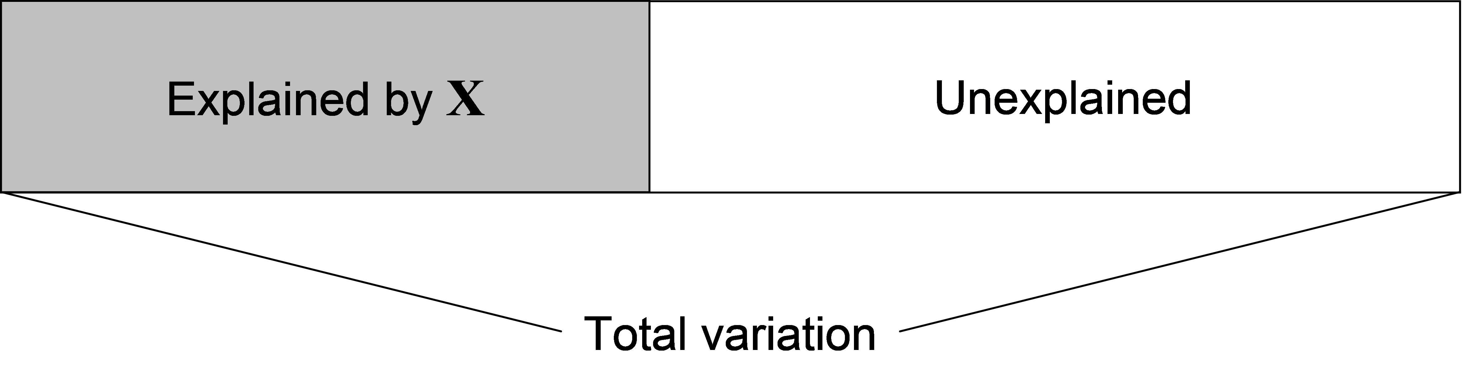
Fig. 4.1. Conceptual diagram of regression as a partitioning of the total variation into a portion that is explained by the predictor variables in matrix X, and a portion that is left unexplained (the residual).
Details of how dbRDA is done are provided by Legendre & Anderson (1999) and McArdle & Anderson (2001) . Maintaining a clear view of the conceptual framework is what matters most (Fig. 4.1), but a thumbnail sketch of the matrix algebra involved in the mechanics of dbRDA is also provided here. Suppose that D is an N × N matrix of dissimilarities (or distances) among samples75. The analysis proceeds through the following steps (Fig. 4.2):
-
From the matrix of dissimilarities, D, calculate matrix A, then Gower’s centred matrix G, as outlined in steps 1 and 2 for doing a PCO (see Fig. 3.1);
-
The total sum of squares ($SS _{ \text{Total}}$) of the full multivariate data cloud is the sum of the diagonal elements (called the “trace” and symbolised here by “tr”) of matrix G, that is, tr(G);
-
From matrix X, calculate the “hat” matrix H = X[X′X]$^ {-1}$X′. This is the matrix derived from the solutions to the normal equations ordinarily used in multiple regression (e.g., Johnson & Wichern (1992) , Neter, Kutner, Nachtsheim et al. (1996) )76;
-
The explained sum of squares for the regression ($SS _{ \text{Regression}}$) is then calculated directly as tr(HGH);
-
The unexplained (or residual) sum of squares is then $SS _{ \text{Residual}} = SS _{ \text{Total}} – SS _{ \text{Regression}}$. This is also able to be calculated directly as tr([I – H]G[I – H]), where I is an N × N identity matrix77.
 Fig. 4.2. Schematic diagram of distance-based redundancy analysis as performed by DISTLM.
Once the partitioning has been done, the proportion of the variation in the multivariate data cloud that is explained by the variables in X is calculated as: $$ R ^ 2 = \frac{ SS _{ \text{Regression}} }{ SS _{ \text{Total}}} \tag{4.1} $$ Furthermore, an appropriate statistic for testing the general null hypothesis of no relationship is: $$ F = \frac{ SS _{ \text{Regression}} / q}{ SS _{ \text{Residual}} / (N - q -1)} \tag{4.2} $$
This is the pseudo-F statistic, as already seen for the ANOVA case in chapter 1 (equation 1.3). It is a direct multivariate analogue of Fisher’s F ratio used in traditional regression. However, when using DISTLM, we do not presume to know the distribution of pseudo-F in equation 4.2, especially for p > 1 and where a non-Euclidean dissimilarity measure has been used as the basis of the analysis. Typical values we might expect for pseudo-F in equation (4.2) if the null hypothesis of no relationship were true can be obtained by randomly re-ordering the sample units in matrix Y (or equivalently, by simultaneously re-ordering the rows and columns of matrix G), while leaving the ordering of samples in matrix X (and H) fixed. For each permutation, a new value of pseudo-F is calculated (F$ ^ \pi$). There is generally going to be a very large number of possible permutations for a regression problem such as this; a total of N! (i.e., N factorial) re-orderings are possible. A large random subset of these will do in order to obtain an exact P-value for the test ( Dwass (1957) ) . The value of pseudo-F obtained with the original ordering of samples is compared with the permutation distribution of F$ ^ \pi$ to calculate a P-value for the test (see equation 1.4 in chapter 1).
If Euclidean distances are used as the basis of the analysis, then DISTLM will fit a traditional linear model of Y versus X, and the resulting F ratio and R$^2$ values will be equivalent to those obtained from:
-
a simple regression (when p = 1 and q = 1);
-
a multiple regression (when p = 1 and q > 1); or
-
a multivariate multiple regression (when p > 1 and q > 1). Traditional multivariate multiple regression is also called redundancy analysis or RDA ( Gittins (1985) , ter Braak (1987) ).
An important remaining difference, however, between the results obtained by DISTLM compared to other software for such cases is that all P-values in DISTLM are obtained by permutation, thus avoiding the usual traditional assumption that errors be normally distributed.
The added flexibility of DISTLM, just as for PERMANOVA, is that any resemblance measure can be used as the basis of the analysis. Note that the “hat” matrix (H) is so-called because, in traditional regression analysis, it provides a projection of the response variables Y onto X ( Johnson & Wichern (1992) ) transforming them to their fitted values, which are commonly denoted by $\hat{\text{\bf Y}}$ . In other words, we obtain fitted values (“y-hat”) by pre-multiplying Y by the hat matrix: $\hat{\text{\bf Y}} = \text{\bf HY}$. Whereas in traditional multivariate multiple regression the explained sum of squares (provided each of the variables in Y are centred on their means) can be written as tr($\hat{\text{\bf Y}}$ $\hat{\text{\bf Y}}^ \prime$ )=tr(HYY$^\prime$H), we achieve the ability to partition variability more generally on the basis of any resemblance matrix simply by replacing YY$^\prime$ in this equation with G ( McArdle & Anderson (2001) ). If Euclidean distances are used in the first place to generate D, then G and YY$^ \prime$ are equivalent78 and DISTLM produces the same partitioning as traditional RDA. However, if D does not contain Euclidean distances, then G and YY$^ \prime$ are not equivalent and tr(HGH) produces the explained sum of squares for dbRDA on the basis of the chosen resemblance measure.
Two further points are worth making here about dbRDA and its implementation in DISTLM.
-
First, as should be clear from the construction of the pseudo-F statistic in equation 4.2, the number of variables in X(q) cannot exceed (N – 1), or we simply run out of residual degrees of freedom! Furthermore, if q = N – 1, then we will find that $R ^ 2$ reaches its maximum at 1.0, meaning the percentage of variation explained is 100%, even if the variables in X are just random numbers! This is a consequence of the fact that $R ^ 2$ always increases with increases in the number of predictor variables. It is always possible to find a linear combination of (N – 1) variables (or axes) that will fit N points perfectly (see the section Mechanics of PCO in chapter 3). Thus, if q is large relative to N, then a more parsimonious model should be sought using appropriate model selection criteria (see the section Building models).
-
Second, the method implemented by DISTLM, like PERMANOVA but in a regression context, provides a true partitioning of the variation in the data cloud, and does not suffer from the problems identified for partial Mantel tests identified by Legendre, Borcard & Peres-Neto (2005) . The partial Mantel-type methods “expand” the resemblance matrix by “unwinding” it to a total of N(N – 1)/2 different dissimilarity units. These are then (unfortunately) treated as independent samples in regression models. In contrast, the units being treated as independent in dbRDA are the original individual samples (the N rows of Y, say), which are the exchangeable units under permutation. Thus, the inherent structure (the correlation among variables and the values within a single sample row) and degree of non-independence among values in the resemblance matrix remain intact under the partitioning and permutation schemes of dbRDA (whether it is being implemented using the PERMANOVA routine or the DISTLM routine), but this is not true for partial Mantel tests79. See the section entitled SS from a distance matrix in chapter 1 for further discussion.
75 If a resemblance matrix of similarities is available instead, then DISTLM in PERMANOVA+ will automatically transform these into dissimilarities; the user need not do this as a separate step.
76 Regression models usually include an intercept term. This is obtained by including a single column of 1’s as the first column in matrix X. DISTLM automatically includes an intercept in all of its models. This amounts to centring the data before analysis and has no effect on the calculations of explained variation.
77 An identity matrix (I) behaves algebraically like a “1” in matrix algebra. It is a square diagonal matrix with 1’s all along its diagonal and zeros elsewhere.
78 This equivalence is noted on p. 426 of Legendre & Legendre (1998) and is also easy to verify by numerical examples.
79 An interesting point worth noting here is to consider how many df are actually available for a multivariate analysis. If p = 1, then we have a total of N independent units. If p > 1, then if all variables were independent of one another, we would have N × p independent units. We do not expect, however, to have independent variables, so, depending on their degree of inter-correlation, we expect the true df for the multivariate system to lie somewhere between N and N × p. The Mantel-type procedure, which treats with N(N – 1)/2 units is generally going to overestimate the true df, or information content of the multivariate system, while PERMANOVA and dbRDA’s use of N is, if anything, an underestimate. This is clearly an area that warrants further research.
4.4 Simple linear regression (Clyde macrofauna)
In our first example of DISTLM, we will examine the relationship between the Shannon diversity (H′) of macrofauna and log copper concentration from benthic sampling at 12 sites along the Garroch Head dumpground in the Firth of Clyde, using simple linear regression. How much of the variation in macrofaunal diversity (Y) is explained by variation in the concentration of copper in the sediment (X)? In this case, p = q = 1, so both Y and X are actually just single vectors containing one variable (rather than being whole matrices). We shall do a DISTLM analysis on the basis of Euclidean distances, which is equivalent to univariate simple linear regression, but where the P-value for the test is obtained using permutations, rather than by using traditional tables.
In PRIMER, open up the environmental data file clev.pri and also the macrofaunal data file clma.pri, which are both located in the ‘Clydemac’ folder of the ‘Examples v6’ directory. Here, we will focus first only on a single predictor variable: copper. Highlight the variable ‘Cu’ and choose Select > Highlighted. Next, transform the variable (for consistency, we shall use the log-transformation suggested by Clarke & Gorley (2006) ), by choosing Tools > Transform(individual) > Expression: log(0.1+V). Rename the transformed variable ‘ln Cu’, and also rename the data sheet containing this variable ln Cu. Next, go to the sheet containing the macrofaunal data clma and choose Analyse > DIVERSE. In the resulting dialog, remove the tick marks from all of the measures (shown under the ‘Other’ tab or the ‘Simpson’ tab), so that the only diversity measure that will be calculated is Shannon’s index H′ (shown under the ‘Shannon’ tab) using Log base $\checkmark$e. Place a tick mark next to $\checkmark$Results to worksheet, then click OK. Rename the resulting data sheet H′. Calculate Euclidean distances among samples on the basis of H′ alone. That is, from the H′ data sheet, choose Analyse > Resemblance > (Analyse between •Samples) & (Measure •Euclidean distance).
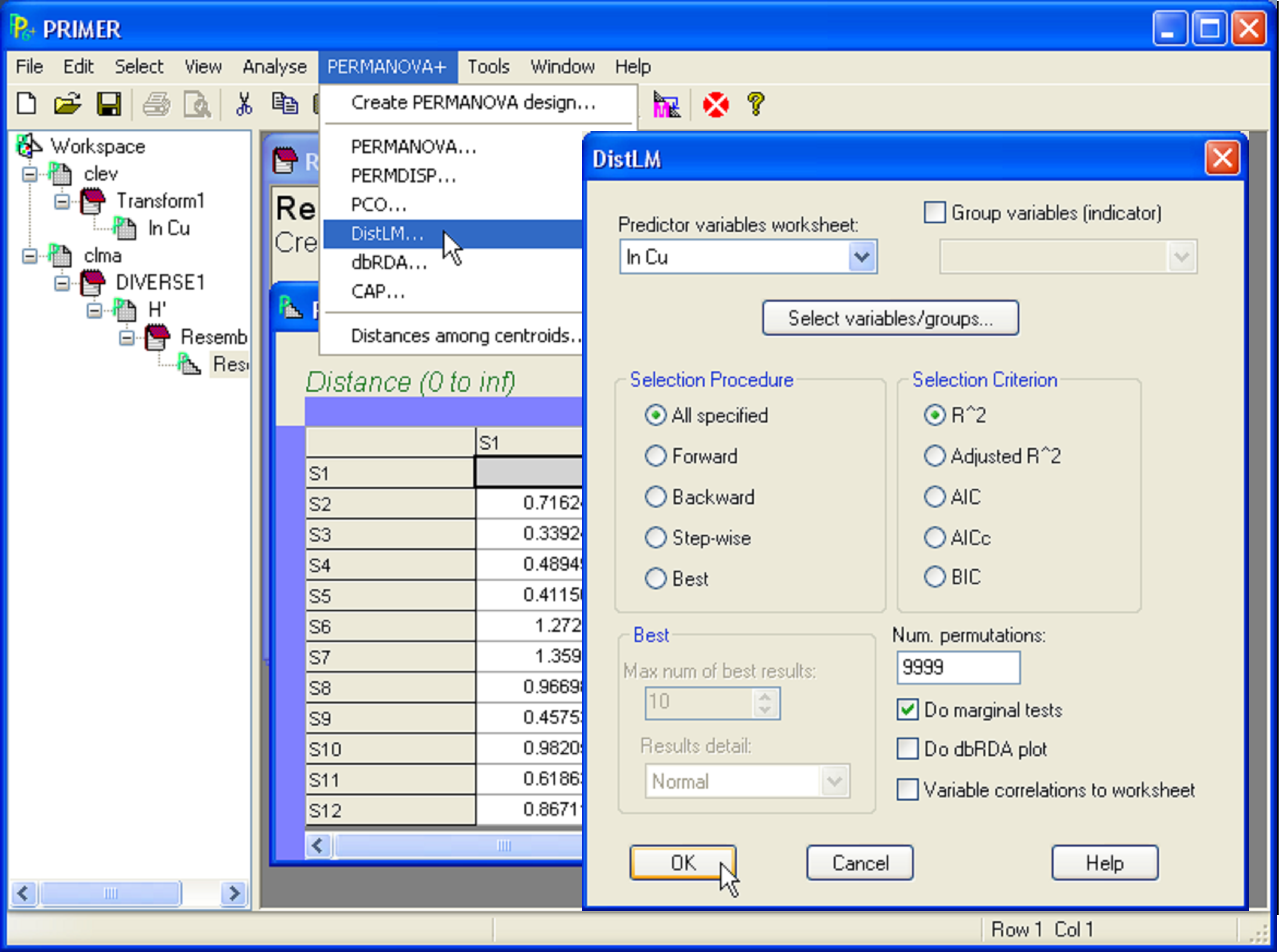
Fig. 4.3. DISTLM procedure for simple linear regression of Clyde macrofaunal diversity (H′) versus log copper concentration (ln Cu).
With the predictor (X) variable(s) in one sheet and the resemblance matrix (arising from the response variable(s) Y) in another, we are now ready to proceed with the analysis. DISTLM, like all of the methods in the PERMANOVA+ add-on, begins from the resemblance matrix. Note that the number and names of the samples in the resemblance matrix have to match precisely the ones listed in the worksheet of predictor variables. They do not necessarily have to be in the same order, but they do have to have the same strict names, so that they can be matched and related to one another directly in the analysis. Choose PERMANOVA+ > DISTLM > (Predictor variables worksheet: ln Cu) & (Selection procedure •All specified) & (Selection criterion •R^2) & (Num. permutations: 9999) (Fig. 4.3).
The results file (Fig. 4.4) shows that the proportion of the variation in Shannon diversity explained by log copper concentrations is quite large ($R ^ 2 = 0.815$, as seen in the column headed ‘Prop.’) and, not surprisingly, statistically significant by permutation (P = 0.0001). Thus, 81.5% of the variation in macrofaunal diversity among these 12 sites (as measured by H′ alone) is explained by variation in log copper concentration. Also shown in the output is the explicit quantitative partitioning: $SS _ \text{Total} = 7.63$ and $SS _ \text{Regression} = 6.22$. As there is only one predictor variable here, the information given under the heading ‘Marginal tests’ (Fig. 4.4) is all that is really needed from the output file. To see a scatterplot for this simple regression case, go to the ln Cu worksheet and choose Tools > Merge > Second worksheet: H′> OK. From this merged data worksheet (called ‘Data1’ by default), choose Analyse > Draftsman Plot > $\checkmark$Correlations to worksheet > OK. The plot shows that H′ decreases strongly with increasing ln Cu and the Pearson linear correlation (r) is -0.903 (Fig. 4.4). Indeed, this checks out with what was given in DISTLM for $R ^2$, as (-0.903)$^2$ = 0.815.
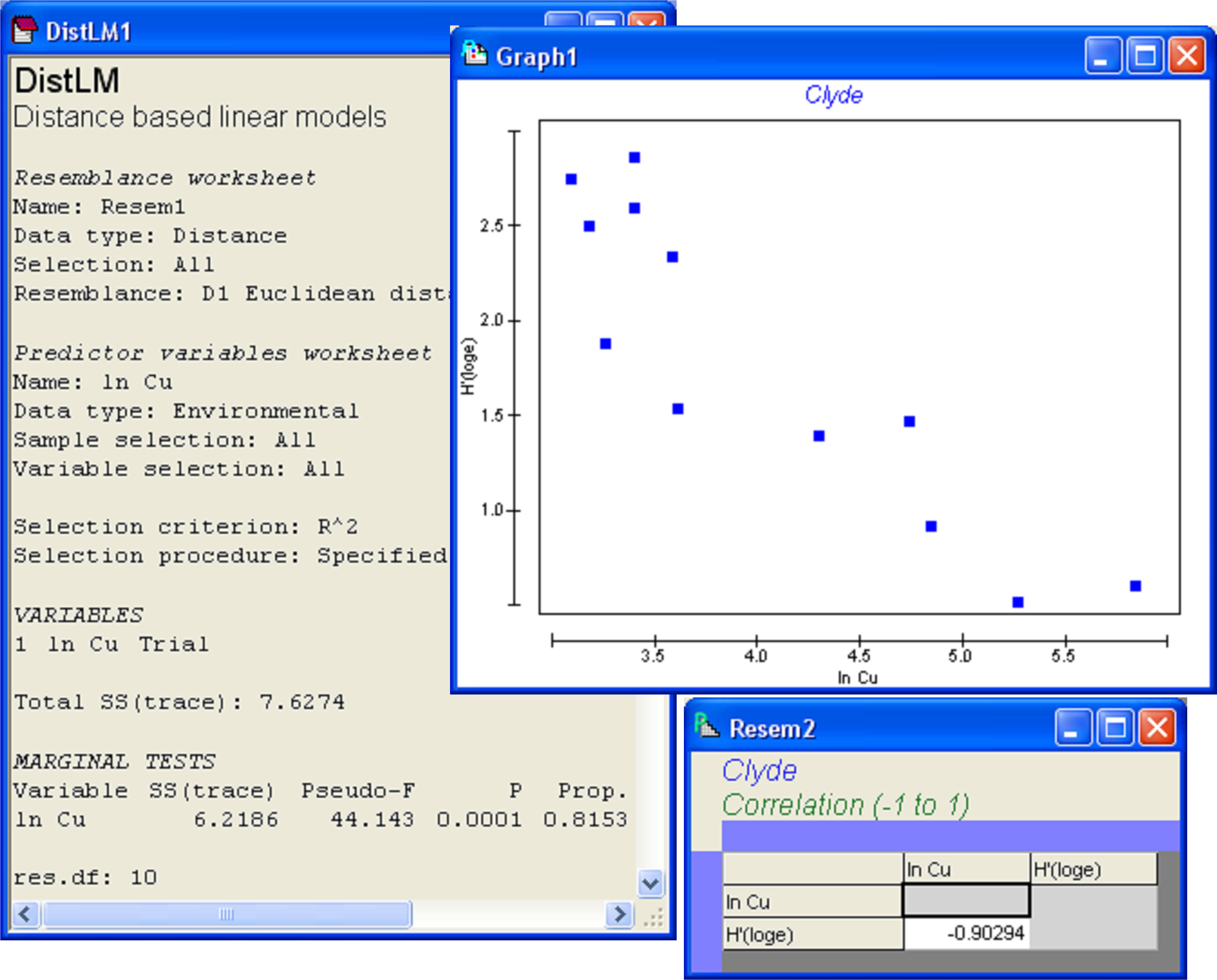
Fig. 4.4. DISTLM results for the regression of diversity of Clyde macrofauna (H′) versus log copper concentration (ln Cu).
4.5 Conditional tests
More generally, when X contains more than one variable, we may also be interested in conditional or partial tests. For example, if X contains two variables X$_1$ and X$_2$, or (more generally) two sets of variables X$_1$ and X$_2$, one may ask: how much of the variation among samples in the resemblance matrix is explained by X$_2$, given that X$_1$ has already been fitted in the model? Usually, the two variables (or sets of variables) are not completely independent of one another, and the degree of correlation between them will result in there being some overlap in the variability that they explain (Fig. 4.5). This means that the amount explained by an individual variable will be different from the amount that it explains after one or more other variables have been fitted. A test of the relationship between a response variable (or multivariate data cloud) and an individual variable alone is called a marginal test, while a test of such a relationship after fitting one or more other variables is called a conditional or partial test. When fitting more than one quantitative variable in a regression-type of context like this, the order of the fit matters.
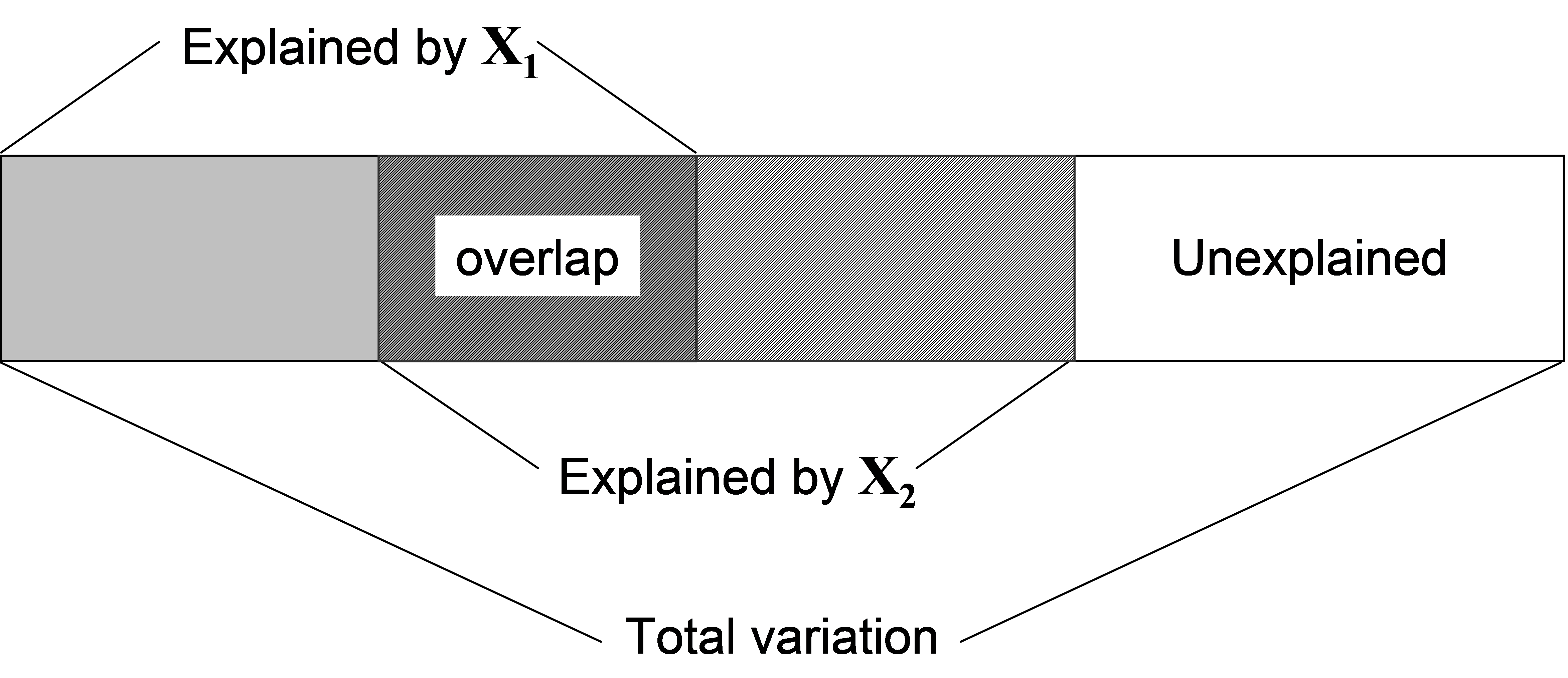 Fig. 4.5. Schematic diagram of partitioning of variation according to two predictor variables (or sets of variables), X1 and X2.
Suppose we wish to test the relationship between the response data cloud and X$_2$, given X$_1$. The variable(s) in X$_1$ in such a case are also sometimes called covariates80. If we consider that the model with both X$_1$ and X$_2$ is called the “full model”, and the model with only X$_1$ is called the “reduced model” (i.e. the model with all terms fitted except the one we are interested in for the conditional test), then the test statistic to use for a conditional test is: $$ F = \frac{ \left( SS _ \text{Full} - SS _ \text{Reduced} \right) / \left( q _ \text{Full} - q _ \text{Reduced} \right) } { \left( SS _ \text{Total} - SS _ \text{Full} \right) / \left( N - q _ \text{Full} - 1 \right) } \tag{4.3} $$ where $SS _ \text{Full}$ and $SS _ \text{Reduced}$ are the explained sum of squares from the full and reduced model regressions, respectively. Also, $q _ \text{Full}$ and $q _ \text{Reduced}$ are the number of variables in X for the full and reduced models, respectively. From Fig. 4.6, it is clear how this statistic isolates only that portion of the variation attributable to the new variable(s) X$_2$ after taking into account what is explained by the other(s) in X$_1$.
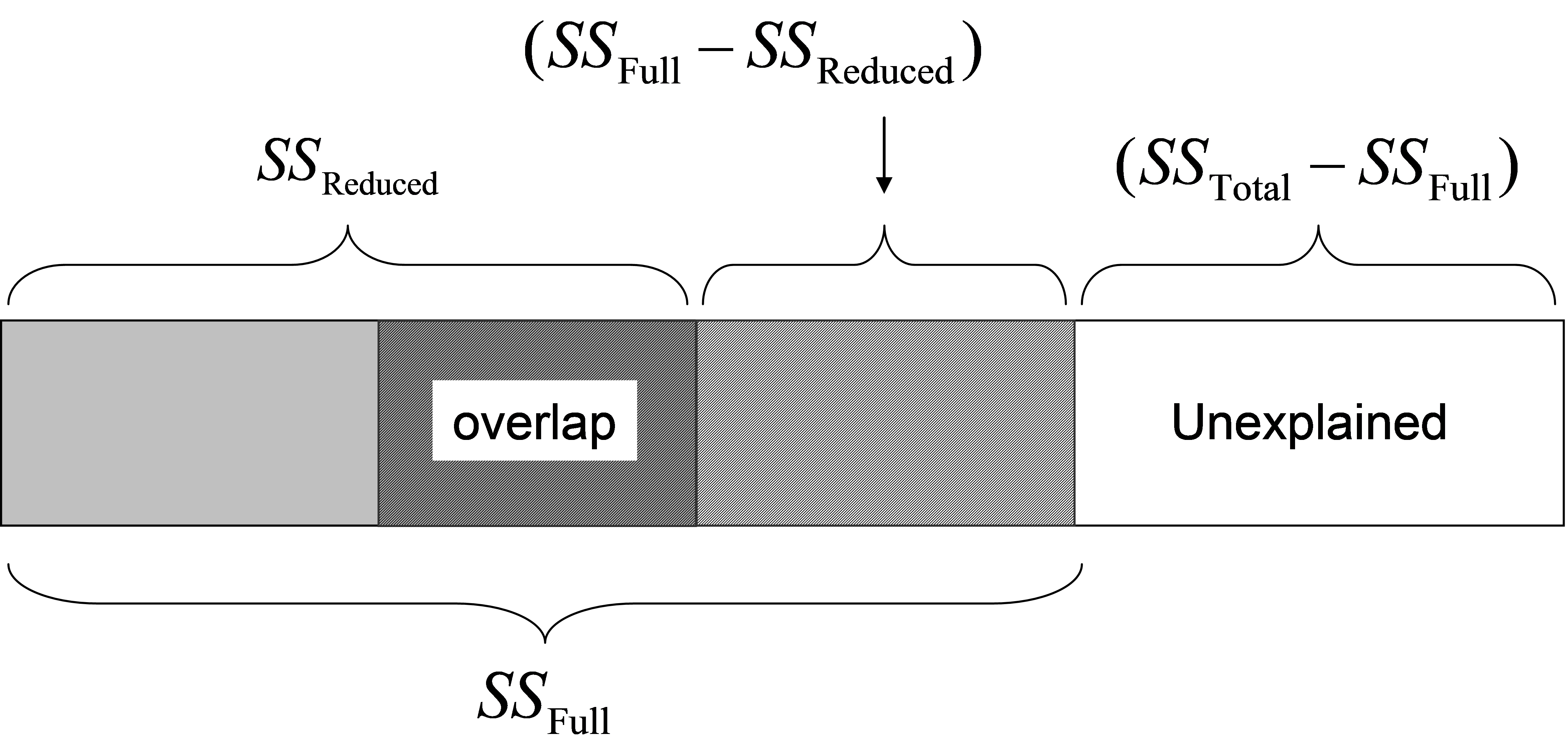 Fig. 4.6. Schematic diagram of partitioning of variation according to two sets of predictor variables, as in Fig. 4.5, but here showing the sums of squares used explicitly by the F ratio in equation (4.3) for the conditional test.
The other consideration for the test is how the permutations should be done under a true null hypothesis. This is a little tricky, because we want any potential relationship between the response data cloud and X$_1$ along with any potential relationship between X$_1$ and X$_2$ to remain intact while we “destroy” any relationship between the response data cloud and X$_2$ under a true null hypothesis. Permuting the samples randomly, as we would for the usual regression case, will not really do here, as this approach will destroy all of these relationships81. What we can do instead is to calculate the residuals of the reduced model (i.e. what is “left over” after fitting X$_1$). By definition, these residuals are independent of X$_1$, and they are therefore exchangeable under a true null hypothesis of no relationship (of the response) with X$_2$. The only other trick is to continue to condition on X$_1$, even under permutation. Thus, with each permutation, we treat the residuals as the response data cloud and calculate pseudo-F as in equation (4.3), in order to ensure that X$_1$ is always taken into account in the analysis. This is required because, interestingly, once we permute the residuals, they will no longer be independent of X$_1$ ( Anderson & Legendre (1999) ; Anderson & Robinson (2001) )! This method of permutation is called permutation of residuals under a reduced model ( Freedman & Lane (1983) ). Anderson & Legendre (1999) showed that this method performed well compared to alternatives in empirical simulations82.
The definition of an exact test was given in chapter 1; for a test to be exact, the rate of type I error (probability of rejecting H$_0$ when it is true) must be equal to the significance level (such as $\alpha = 0.05$) that is chosen a priori. Permutation of residuals under a reduced model does not provide an exact test, but it is asymptotically exact – that is, its type I error approaches $\alpha$ with increases in the sample size, N. The reason it is not exact is because we must estimate the relationship between the data cloud and X$_1$ to get the residuals, and this is (necessarily) imperfect – the residuals only approximate the true errors. If we knew the true errors, given X$_1$, then we would have an exact test. Clearly, the estimation gets better the greater the sample size and, as shown by Anderson & Robinson (2001) , permutation of residuals under a reduced model is as close as we can get to this conceptually exact test.
There are (at least) two ways that the outcome of a conditional test can surprise the user, given results seen in marginal tests for individual variables:
-
Suppose the marginal test of Y versus X$_2$ is statistically significant. The conditional test of Y versus X$_2$ can be found to be non-significant, after taking into account the relationship between Y and X$_1$.
-
Suppose the marginal test of Y versus X$_2$ is not statistically significant. The conditional test of Y versus X$_2$ can be found, nevertheless, to be highly significant, after taking into account the relationship between Y and X$_1$.
The first of these scenarios is somewhat straightforward to visualise, by reference to the graphical representation in Fig. 4.7 (left-hand side). Clearly, if there is a great deal of overlap in the variability of Y explained by X$_1$ and X$_2$, then the fitting of X$_1$ can effectively “wipe-out” a large portion of the variation in Y explained by X$_2$, thus rendering it non-significant. On the other hand, the second of these scenarios is perhaps more perplexing: how can X$_2$ suddenly become important in explaining the variation in Y after fitting X$_1$ if it was originally deemed unimportant when considered alone in the marginal test? The graphical representation in Fig. 4.7 (right-hand side) should help to clarify this scenario: here, although X$_2$ explains only a small portion of the variation in Y on its own, its component nevertheless becomes a significant and substantial proportion of what is left (compared to the residual) once X$_1$ is taken into account. These relationships become more complex with greater numbers of predictor variables (whether considered individually or in sets) and are in fact multi-dimensional, which cannot be easily drawn schematically. The primary take-home message is not to expect the order of the variables being fitted in a sequential model, nor the associated sequential conditional tests, necessarily to reflect the relative importance of the variables shown by the marginal tests.
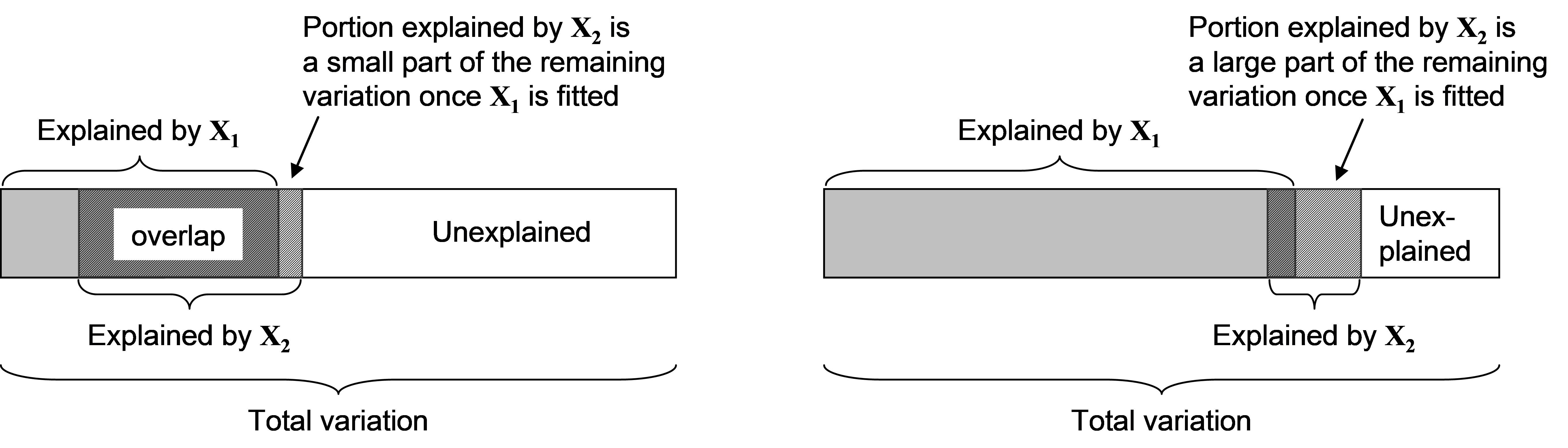
Fig. 4.7. Schematic diagrams showing two scenarios (left and right) where the conditional test of Y versus X$_2$ given X$_1$ can differ substantially from the outcome of the marginal test of Y versus X$_2$ alone.
80 See also the section entitled Designs with covariates in chapter 1.
81 But see the discussion in Manly (2006) and also Anderson & Robinson (2001) , who show that this approach can still give reasonable results in some cases, provided there are no outliers in the covariates.
82 See the section entitled Methods of permutation in chapter 1 on PERMANOVA for more about permutation of residuals under a reduced model.
4.6 (Holdfast invertebrates)
To demonstrate conditional tests in DISTLM, we will consider the number of species inhabiting holdfasts of the kelp Ecklonia radiata in the dataset from New Zealand, located in the file hold.pri in the ‘HoldNZ’ folder of the ‘Examples add-on’ directory. These multivariate data were analysed in the section entitled Designs with covariates in chapter 1. Due to the well-known species-area relationship in ecology, we expect the number of species to increase with the volume (size) of the holdfast ( Smith, Simpson & Cairns (1996) , Anderson, Diebel, Blom et al. (2005) , Anderson, Millar, Blom et al. (2005) ). In addition, the density of the kelp forest surrounding a particular kelp plant might also affect the number of species able to immigrate or emigrate to/from the holdfast ( Goodsell & Connell (2002) ) and depth can also play a role in structuring holdfast communities ( Coleman, Vytopil, Goodsell et al. (2007) ). Volume (in ml), density of surrounding Ecklonia plants (per m$^2$) and depth (in m) were all measured as part of this study and are contained in the file holdenv.pri. The associated draftsman plot (Fig. 1.45) shows that these variables are reasonably evenly distributed across their range (see Assumptions & diagnostics).
Here, we will focus on the number of species of molluscs only, as members of this phylum were all identified down to species level. Open the file hold.pri in PRIMER, select the molluscan species only and duplicate these into their own sheet, named molluscs, as shown in Fig. 1.27 in the section entitled Nested designs of chapter 1. Choose Analyse > DIVERSE and retain only the tick mark next to $\checkmark$Total species: S on the ‘Other’ tab, but remove all others. Also choose to get $\checkmark$Results to worksheet and name the resulting sheet No.species. This will be the (in this case univariate) response variable for the analysis. Calculate a Euclidean distance matrix among samples on the basis of this variable. Next, open up the holdenv.pri file in PRIMER. Here we shall focus on running the analysis on only two predictor variables: volume and density, asking the specific question: does density explain a significant portion of the variation in the number of species of molluscs after volume is taken into account? Do this by choosing PERMANOVA+ > DISTLM > (Predictor variables worksheet: holdenv) and click on the button marked ‘Select variables/groups’. This opens up a ‘Selection’ dialog where you can choose to force the inclusion or exclusion of particular variables from the model and you can also change the order in which the variables (listed in the ‘Available’ column) are fitted. Choose to exclude depth for the moment and to fit volume first, followed by density (see Fig. 4.8). Back in the DISTLM dialog, choose (Selection procedure •All specified) & (Selection criterion •R^2) & (Num. permutations: 9999).
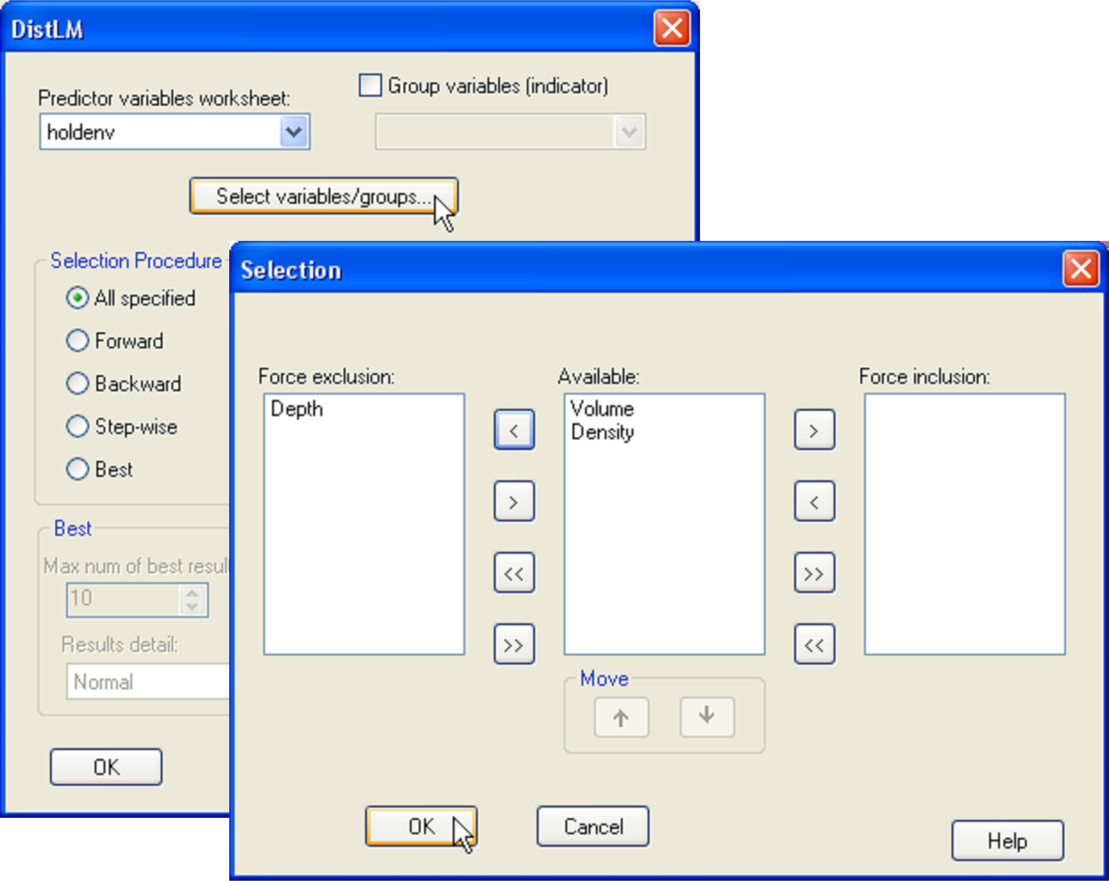
Fig. 4.8. Dialog in DISTLM for specifying a model with two variables, volume and density (in that order), but excluding the variable of depth.
The results (Fig. 4.9) show first the marginal tests of how much each variable explains when taken alone, ignoring all other variables. Here, we see that volume explains a significant amount of about 32.8% of the variation in the number of mollusc species (P = 0.0001). Density, when considered alone, only explains about 5.7% of the variation, but this small amount is nevertheless found to be statistically significant when tested by permutation (P = 0.037). Note that these marginal tests do not include any corrections for multiple testing. Although this is not such a big issue in the present example, where there are only two marginal tests, clearly the probability of rejecting a null hypothesis by chance will increase the more tests we do, and if there are a lot of predictor variables, the user may wish to adjust the level of significance at which individual tests reject their null hypothesis. The philosophy taken here, as in the case of multiple pair-wise tests in the PERMANOVA routine, is that the permutation approach provides an exact test for each of these individual hypotheses. It is then up to the user to decide whether or not to apply subsequent corrections, if any, to guard against the potential inflation of overall rates of error.
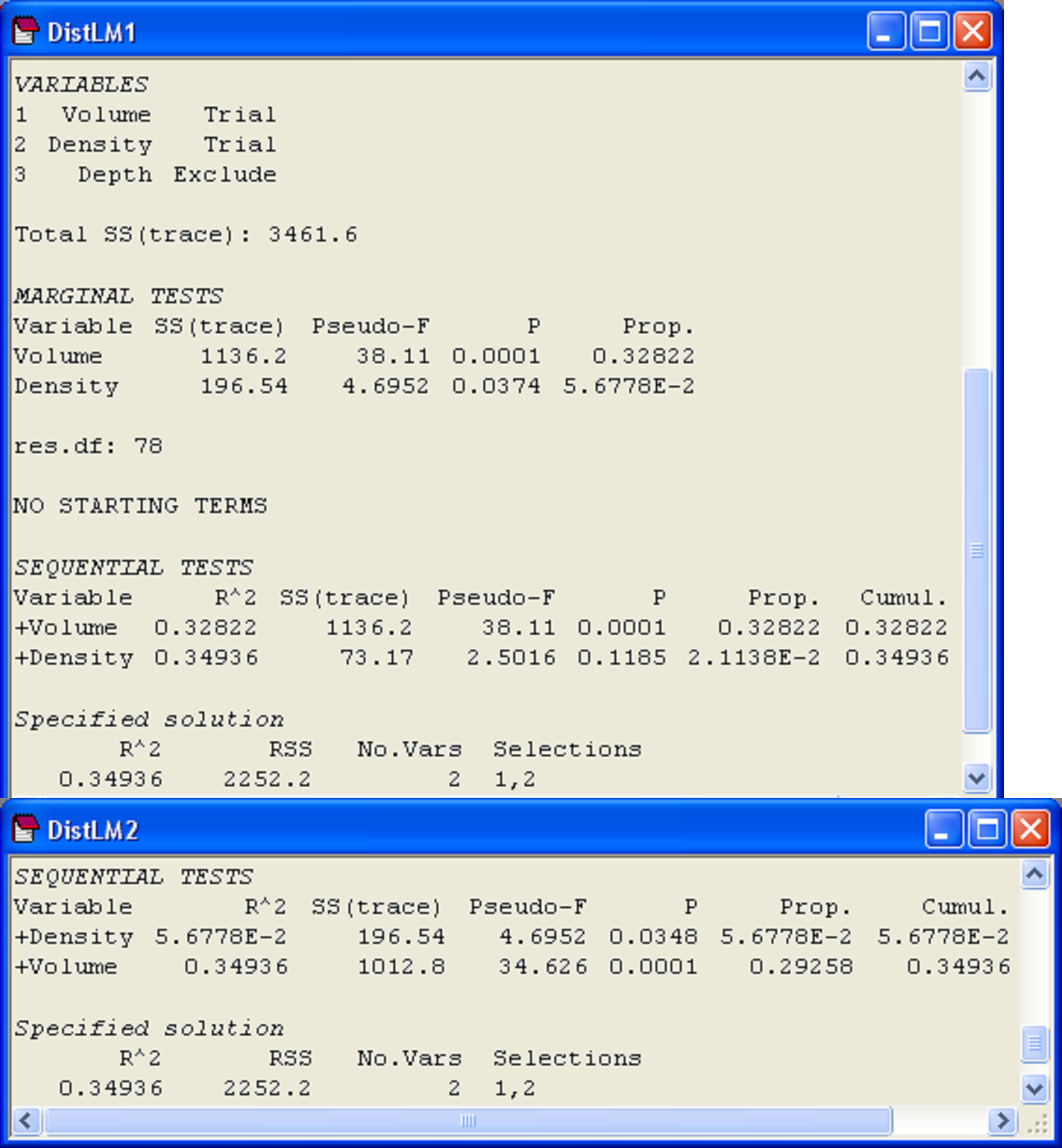
Fig. 4.9. Results from DISTLM obtained by first fitting volume followed by density (‘DistLM1’), including marginal tests, and then by fitting density followed by volume (‘DistLM2’).
Following the marginal tests in the output file, there is a section that contains sequential tests. These are the conditional tests of individual variables done in the order specified. All variables appearing above a particular variable are fitted as covariates, and each test examines whether adding that particular variable contributes significantly to the explained variation. In our case, we have the test of whether density adds a significant amount to the explained variation, given that volume has already been included in the model. These sequential conditional tests correspond directly to the notion of Type I SS met in chapter 1 (e.g., see Fig. 1.41). That is, we fit variable 1, then variable 2 given variable 1, then variable 3 given variables 1 and 2, and so on. In the present example (Fig. 4.9, ‘DistLM1’), density adds only about an additional 2.1% to the explained variation once volume has been fitted, and this is not statistically significant (P = 0.12). The column labeled ‘Prop.’ in the section of the output entitled ‘Sequential tests’ indicates the increase in the proportion of explained variation attributable to each variable that is added, and the column labeled ‘Cumul.’ provides a running cumulative total. For this example, these two variables together explained 34.9% of the variation in number of mollusc species in the holdfasts.
We can re-run this analysis and change the order in which the variables are fitted. This is done by clicking on particular variables and using the ‘Move’ arrows under the names of variables listed in the ‘Available’ column of the ‘Selection’ dialog box within DISTLM. There is no need to include marginal tests again, so we can also remove the tick in front of ‘Do marginal tests’ in the ordinary DISTLM dialog. When we fit density first, followed by volume, it is not at all surprising to find that: (i) volume explains a significant proportion of variation even after fitting density and (ii) the variation explained by both variables together remains the same, at 34.9% (Fig. 4.9, ‘DistLM2’).
4.7 Assumptions & diagnostics
Thus far, we have only done examples for a univariate response variable in Euclidean space, using DISTLM to fit linear models, but with tests being done by permutation. However, the fact that any resemblance measure can be used as the basis of the analysis in dbRDA yields considerable flexibility in terms of modeling. In traditional regression and RDA, the fitted values are a linear combination of the variables in X. So, the relationship between the multivariate data Y and predictor variables X is assumed to be linear for the purposes of modeling. In dbRDA, however, the relationship being modeled between Y and X variables is more complex and depends on the chosen resemblance measure. Another way to describe dbRDA is that it is a traditional RDA done on the PCO axes83 from a resemblance matrix, rather than on the original Y variables. Thus, in dbRDA, we effectively assume a linear relationship between the PCO axes derived from the resemblance matrix and the variables in X for purposes of modeling ( Legendre & Anderson (1999) ). In many cases, this is quite appropriate provided the resemblance measure used as the basis of the analysis is a sensible one for the data. By “sensible”, we mean that the resemblance measure describes multivariate variation in a way that emphasises the features of the data that are of interest (e.g., changes in composition, relative abundance, etc.) for specific hypotheses postulated by the user. Note, for example, that if one were to perform dbRDA on a chi-squared distance matrix, then this will assume unimodal relationships between Y and X, as is done in canonical correspondence analysis (CCA, ter Braak (1986a) , ter Braak (1986b) )84. Clearly dbRDA goes beyond what either RDA or CCA can provide, by allowing any resemblance measure (e.g., Bray-Curtis, Manhattan, etc.) to define multivariate variation. In addition, once a given resemblance measure has been chosen, many other kinds of non-linear relationships between the PCO axes and X can be modeled by introducing polynomials of the variables in X, if desired (e.g., Makarenkov & Legendre (2002) ).
Although dbRDA does provide quite impressive flexibility with respect to the response variables (Y), it pays to spend some time with the X variables to examine their distributions and the relationships among them, as these are being treated in the same way in dbRDA as they would for any linear multiple regression model. Although DISTLM does not make any explicit assumptions about the distributions of the X variables, they should nevertheless be reasonable for purposes of linear modeling – they should not be heavily skewed or contain extreme outliers. It is a very good idea, therefore, to examine the X variables using a draftsman plot in PRIMER and to transform them (individually if necessary) to avoid skewness before proceeding.
The issue of multi-collinearity – strong inter-correlations among the X variables – is also something to watch out for in dbRDA, as it is for RDA or multiple regression (e.g., Neter, Kutner, Nachtsheim et al. (1996) ). If two variables in X are very highly co-linear (with correlation |r| ≥ 0.95, for example), then they contain effectively the same information and are redundant for purposes of the analysis. A redundant variable should be dropped before proceeding (keeping in mind that the variable which is retained for modeling may of course simply be acting as a proxy for the one that was dropped). Once again, PRIMER’s Draftsman Plot tool will provide useful direct information about multi-collinearity among the variables in X. See pp. 122-123 of chapter 11 in Clarke & Gorley (2006) , for example, which demonstrate how to use the Draftsman Plot tool to identify skewness and multi-collinearity for a set of environmental variables.
In traditional multiple regression, the errors are assumed to be independent and identically distributed (i.i.d.) as normal random variables. DISTLM uses permutations to test hypotheses, however, so normality is not assumed. For a permutation test in regression, if we consider that the null hypothesis is true and Y and X are not related to one another, then the matching of a particular row of Y (where rows identify the samples, as in Fig. 4.2) with a particular row of X does not matter, and we can order the 1 to N rows of Y (or, equivalently, the rows and columns of matrix D) in any way we wish (e.g., Manly (2006) ). Thus, all that is assumed is that the sample rows are exchangeable under a true null hypothesis. For conditional tests, we assume that the residuals obtained after fitting covariates are exchangeable under a true null hypothesis. This means, more particularly, that we assume that the linear model being used to fit the covariate(s) to multivariate data in the space of the resemblance measure is appropriate and that the errors (estimated by the residuals from this model) have homogeneous dispersions in that space, so they are exchangeable.
83 Being careful, that is, to do all computations on the axes associated with positive and negative eigenvalues separately, and combining them only when they are squared (e.g., as sums of squares). Axes corresponding to the negative eigenvalues contribute negatively in the squared terms. See chapter 3 regarding negative eigenvalues and McArdle & Anderson (2001) for more details.
84 If the user performs dbRDA on the basis of the chi-squared distance measure, the results will produce patterns highly similar to those obtained using CCA. Any differences will be due to the intrinsic weights used in CCA. See ter Braak (1987) , Legendre & Legendre (1998) and Legendre & Gallagher (2001) for details regarding the differences between CCA and RDA and the algebraic formulations for these two approaches.
4.8 Building models
In many situations, a scientist may have measured a large number of predictor variables that could be potentially important, and interest lies in determining which ones are best at explaining variation in the response data cloud and also whether particular combinations of variables, working together, do a better job than other combinations in this respect. More specifically, one may wish to build a model for the response data cloud, using the best possible combination of predictor variables available. There are two primary issues one is faced with when trying to build models in this way: first, what criterion should be used to identify a “good” model and second, what procedure should one use to select the variables on the basis of said criterion?
In addition to providing tests of hypotheses for specific regression-style problems, DISTLM also provides the user with a flexible model-building tool. A suite of selection procedures and selection criteria are available, as seen in the DISTLM dialog box and described below.
Selection procedures
-
All specified will simply fit all of the variables in the predictor variables worksheet, either in the order in which they appear in the worksheet (by default) or in the order given explicitly under the ‘Available’ column in the ‘Selection’ dialog. The ‘Selection’ dialog can also be used to force the exclusion or inclusion of certain variables from this or any of the other selection procedures as well.
-
Forward selection begins with a null model, containing no predictor variables. The predictor variable with the best value for the selection criterion is chosen first, followed by the variable that, together with the first, improves the selection criterion the most, and so on. Forward selection therefore adds one variable at a time to the model, choosing the variable at each step which results in the greatest improvement in the value of the selection criterion. At each step, the conditional test associated with adding that variable to the model is also done. The procedure stops when there is no further possible improvement in the selection criterion.
-
Backward elimination begins with a full model, containing all of the predictor variables. The variable which, when removed, results in the greatest improvement in the selection criterion is eliminated first. The conditional test associated with removing each variable is also done at each step. Variables are eliminated from the model sequentially, one at a time, until no further improvement in the criterion can be achieved.
-
Step-wise begins with a null model, like forward selection. First, it seeks to add a variable that will improve the selection criterion. It continues in this fashion, but what distinguishes it from forward selection is that, after every step, it attempts to improve the criterion by removing a term. This approach is therefore like doing a forward selection, followed by a possible backward elimination at every step. The conditional test associated with either the addition or removal of a given variable is done at each step. The procedure stops when no improvements in the selection criterion can be made by either adding or deleting a term. Forward selection is often criticised because it does not allow removal of a term, once it is in the model. The rationale of the step-wise approach responds directly to this criticism.
-
Best is a procedure which examines the value of the selection criterion for all possible combinations of predictor variables. One can choose the level of detail provided in the output file as ‘Normal’, ‘Brief’ or ‘Detailed’, which mirrors similar choices to be made when running the BEST procedure in PRIMER (see chapter 11 in Clarke & Gorley (2006) ). The default output from the Best selection procedure in DISTLM is to provide the best 1-variable model, the best 2-variable model, and so on, on the basis of the chosen selection criterion. The overall 10 best models are also provided (by default) in the output, but this number can be increased if desired. Be aware that for large numbers of predictor variables, the time required to fit all possible models can be prohibitive.
Selection criteria
-
$R^2$ is simply the proportion of explained variation for the model, shown in equation (4.1). Clearly, we should wish for models that have good explanatory power and so, arguably, the larger the value of $R^2$, the better the model. The main drawback to using this as a selection criterion is that, as already noted, its value simply increases with increases in the number of predictor variables. Thus, the model containing all q variables will always be chosen as the best one. This ignores the concept of parsimony, where we wish to obtain a model having good explanatory power that is, nevertheless, as simple as possible (i.e. having as few predictor variables as are really useful).
-
Adjusted $R^2$ provides a more useful criterion than $R^2$ for model selection. We may not wish to include predictor variables in the model if they add no more to the explained sum of squares than would be expected by adding some random variable. Adjusted $R^2$ takes into account the number of parameters (variables) in the model and is defined as: $$ R ^ 2 _ {\text{Adjusted}} = 1 - \frac{ SS _ {\text{Residual}} / \left( N - \nu \right) } { SS _ {\text{Total}} / \left( N - 1 \right) } \tag{4.4} $$ where $\nu$ is the number of parameters in the model (e.g., for the full model with all q variables, we would have $\nu = q+1$, as we are also fitting an intercept as a separate parameter). Adjusted $R^2$ will only increase with decreases in the residual mean square, as the total sum of squares is constant. If adding a variable increases the value of $\nu$ without sufficiently reducing the value of $SS _ {\text{Residual}}$, then adjusted $R^2$ will go down and the variable is not worth including in the model.
-
AIC is an acronym for “An Information Criterion”, and was first described by Akaike (1973) . The criterion comes from likelihood theory and is defined as: $$ AIC = -2 l + 2 \nu \tag{4.5} $$ where $l$ is the log-likelihood associated with a model having $\nu$ parameters. Unlike $R^2$ and adjusted $R^2$, smaller values of AIC indicate a better model. The formulation of AIC from normal theory in the univariate case (e.g., see Seber & Lee (2003) ) can also be written as: $$ AIC = N \log \left( SS _ { \text{Residual}} / N \right) + 2 \nu \tag{4.6} $$ DISTLM uses a distance-based multivariate analogue to this univariate criterion, by simply inserting the $SS _ {\text{Residual}}$ from the partitioning (as is used in the construction of pseudo-F) directly into equation (4.6). Although no explicit qualities of statistical likelihood, per se, are necessarily associated with the use of AIC in this form, we see no reason why this directly analogous function should not provide a reasonable approach. Unlike $R^2$, the value of AIC will not continue to get better with increases in the number of predictor variables in the model. The “$+ 2 \nu$” term effectively adds a “penalty” for increases in the number of predictor variables.
-
AIC$_c$ is a modification of the AIC criterion that was developed to handle situations where the number of samples (N) is small relative to the number of predictor variables (q). AIC was found to perform rather poorly in these situations ( Sugiura (1978) , Sakamoto, Ishiguro & Kitigawa (1986) , Hurvich & Tsai (1989) ). AIC$_c$ is calculated as: $$ AIC _ c = N \log \left( SS _ { \text{Residual}} / N \right) + 2 \nu \left( N / \left( N - \nu - 1 \right) \right) \tag{4.7} $$
In essence, the usual AIC penalty term ($+2 \nu$) has been adjusted by multiplying it by the following correction factor: (N / (N – $\nu$ – 1)). Burnham & Anderson (2002) recommend, in the analysis of a univariate response variable, that AIC$_c$ should be used instead of AIC whenever the ratio N / $\nu$ is small. They further suggest that a ratio of (say) N / $\nu$ < 40 should be considered as “small”! As the use of information criteria such as this in multivariate analysis (including based on resemblance matrices) is still very much in its infancy, we shall make no specific recommendations about this at present; further research and simulation studies are clearly needed. -
BIC, an acronym for “Bayesian Information Criterion” ( Schwarz (1978) ), is much like AIC in flavour (it is not actually Bayesian in a strict sense). Smaller values of BIC also indicate a better model. The difference is that it includes a more severe penalty for the inclusion of extraneous predictor variables. Namely, it replaces the “$+2 \nu$” in equation (4.6) with “$+ \log(N) \nu$” instead. In the DISTLM context, it is calculated as: $$ BIC = N \log \left( SS _ { \text{Residual}} / N \right) + \log \left( N \right) \nu \tag{4.8} $$ For any data set having a sample size of N ≥ 8, then log(N) > 2, and the BIC penalty for including variables in the model will be larger (so more strict) than the AIC penalty.
Depending on the resemblance measure used (and, to perhaps a lesser extent, the scales of the original response variables), it is possible for AIC (or AIC$_c$ or BIC) to be negative for a given model. This is caused, not by the model having a negative residual sum of squares, but rather by $SS _ {\text{Residual}}$ being less than 1.0 in value. When the log is taken of a value less than 1.0, the result is a negative number. However, in these cases (as in all others), smaller values of AIC (or AIC$_c$ or BIC) still correspond to a better model.
Although there are other model selection criteria, we included in DISTLM the ones which presently seem to have the greatest general following in the literature (e.g., Burnham & Anderson (2002) ). For example, Godinez-Dominguez & Freire (2003) used a multivariate analogue to AIC in order to choose among competing models in a multivariate canonical correspondence analysis (CCA). However, the properties and behaviour of these proposed criteria are still largely unknown in the context of dbRDA, especially with multiple response variables ($\rho$ > 1) and for non-Euclidean resemblance measures. More research in this area is certainly required. In the context of univariate model selection, AIC is known to be a rather generous criterion, and will tend to err on the side of including rather too many predictor variables; that is, to “overfit” (e.g., Nishii (1984) , Zhang (1992) , Seber & Lee (2003) ). On the other hand, trials using BIC suggest it may be a bit too severe, requiring the removal of rather too many potentially useful variables. Thus, we suggest that if the use of AIC and BIC yield similar results for a given dataset, then you are probably on the right track! One possibility is to plot a scatter-plot of the AIC and BIC values for the top 20 or so models obtained for a given dataset and see which models fall in the lower left-hand corner (that is, those which have relatively low values using either of these criteria). These are the ones that should be considered as the best current contenders for a parsimonious model. An example of this type of approach is given in an analysis of the Ekofisk macrofauna below.
4.9 Cautionary notes
Before proceeding, a few cautionary notes are appropriate with respect to building models. First, the procedures of forward selection, backward elimination and step-wise selection are in no way guaranteed to find the best overall model. Second, even if the search for the “best” overall model is done, the result will depend on which selection criterion is used (adjusted R$^2$, AIC, AIC$_c$ or BIC). Third, DISTLM fits a linear combination of the X variables, which may or may not be appropriate in a given situation (e.g., see the section on Linkage trees in chapter 11 of Clarke & Gorley (2006) ). As a consequence, it is certainly always appropriate to spend some time with the X variables doing some diagnostic plots and checking out their distributions and relationships with one another as a preliminary step. Fourth, the particular predictor variables that are chosen in a model should not be interpreted as being necessarily causative85. The variables chosen may be acting as proxies for some other important variables that either were not measured or were omitted from the model for reasons of parsimony. Finally, it is not appropriate to use a model selection procedure and then to take the resulting model and test for its significance in explaining variability. This approach uses circular and therefore invalid logic, because it is already the purposeful job of the model selection procedure to select useful explanatory variables. To create a valid test, the inherent bias associated with model selection would need to be taken into account by performing the selection procedure anew with each permutation. Such a test would require a great deal of computational time and is not currently available in DISTLM86. In sum, model-building using the DISTLM tool should generally be viewed as an exploratory hypothesis-generating activity, rather than a definitive method for finding the one “true” model.
85 Unless a predictor variable has been expressly manipulated experimentally in a structured and controlled way to allow causative inferences, that is.
86 The approach of including the selection procedure as part of the test is, however, available for examining non-parametric relationships between resemblance matrices as part of PRIMER’s BEST routine. See pp. 124-125 in chapter 11 of Clarke & Gorley (2006) for details.
4.10 (Ekofisk macrofauna)
We shall now use the DISTLM tool to identify potential parsimonious models for benthic macrofauna near the Ekofisk oil platform in response to several measured environmental variables. The response data (in file ekma.pri in the ‘Ekofisk’ folder of the ‘Examples v6’ directory) consist of abundances of p = 173 species from 3 grab samples at each of N = 39 sites in a 5-spoke radial design (see Fig. 10.6a in Clarke & Warwick (2001) ). Also measured were q = 10 environmental variables (ekev.xls) at each site: Distance (from the oil platform), THC (total hydrocarbons), Redox, % Mud, Phi mean (another grain-size characteristic), and concentrations of several heavy metals: Ba, Sr, Cu, Pb and Ni.
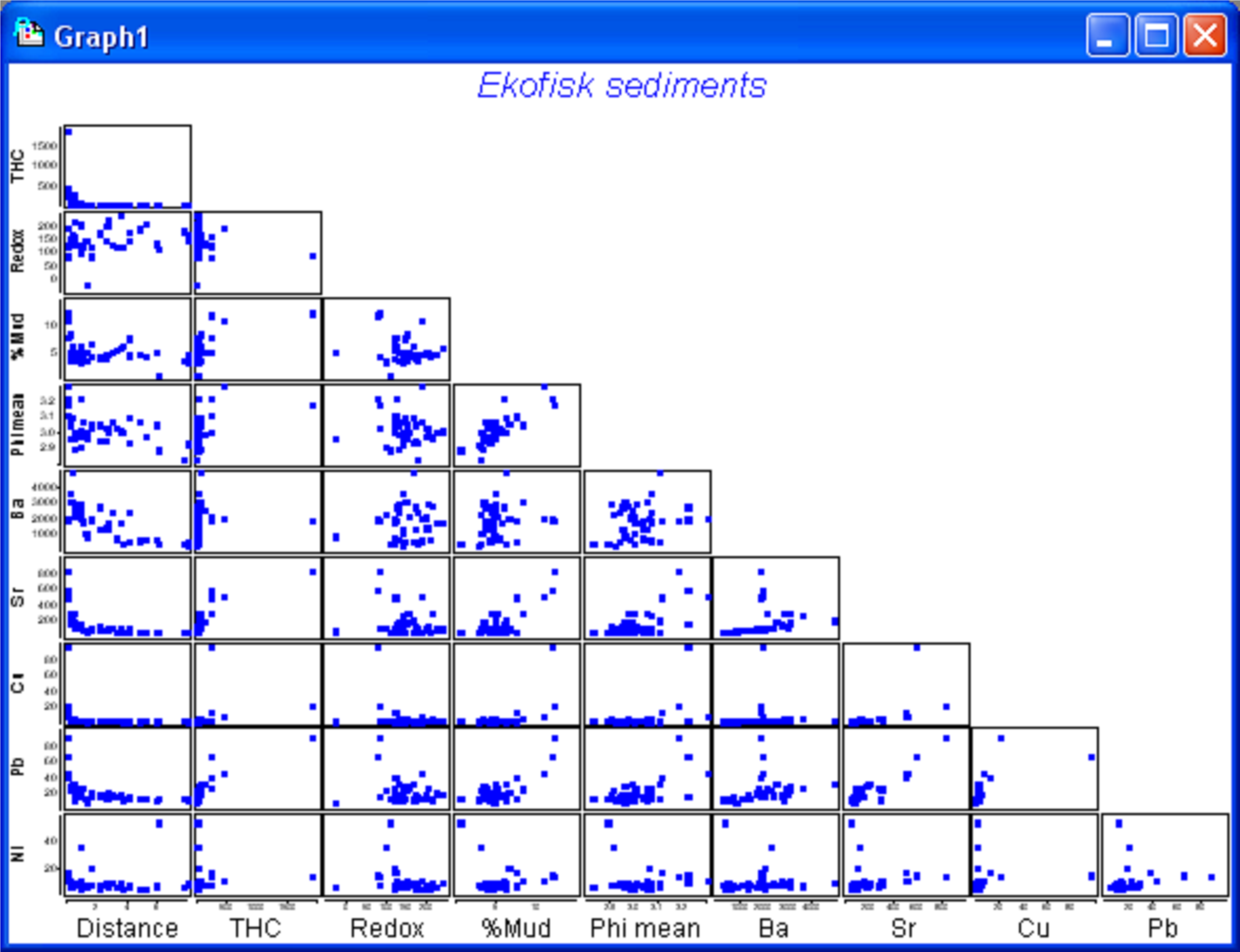
Fig. 4.10. Draftsman plot for the untransformed Ekofisk sediment variables.
We begin by considering some diagnostics for the environmental variables. A draftsman plot indicates that several of the variables show a great deal of right-skewness (Fig. 4.10). The following transformations seemed to do a reasonable job of evening things out: a log transformation for THC, Cu, Pb and Ni, a fourth-root transformation for Distance and % Mud, and a square-root transformation for Ba and Sr. No transformation seems to be necessary for either Redox or Phi mean (Fig. 4.10), the latter already being on a log scale. Transformations were done by highlighting (not selecting) the columns for THC, Cu, Pb and Ni and using Tools > Transform(individual) > (Expression: log(V)) & ($\checkmark$Rename variables). The procedure was then repeated on the resulting data file, first using (Expression: (V)^0.25) on the highlighted columns of Distance and % Mud, and then using (Expression: sqr(V)) on the highlighted columns of Ba and Sr. For future reference, rename the data file containing all of the transformed variables ekevt and save it as ekevt.pri. By choosing Analyse > Draftsman Plot > ($\checkmark$Correlations to worksheet) we are able to examine not just the bivariate distributions of these transformed variables but also their correlation structure (Fig. 4.11).
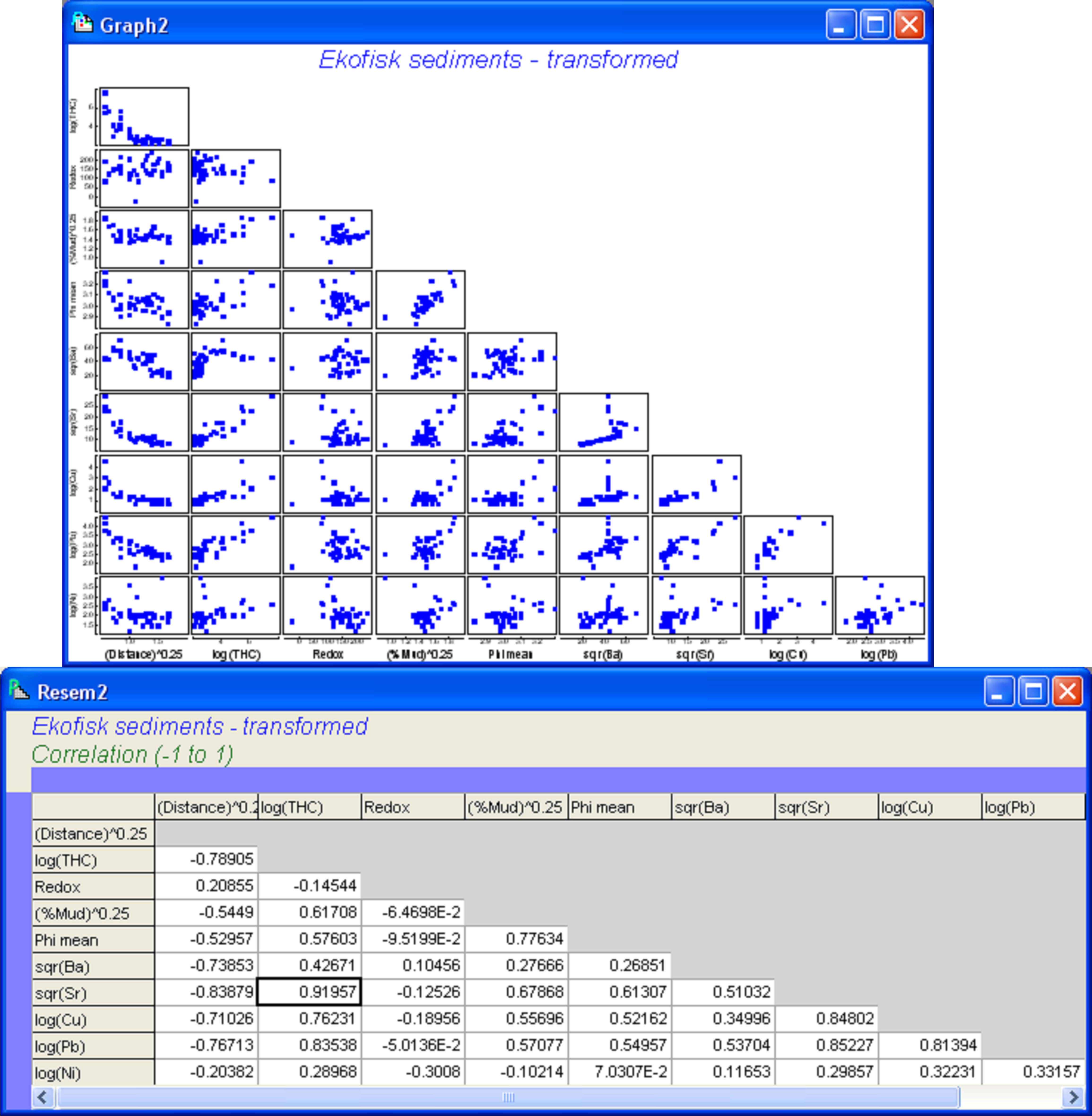
Fig. 4.11. Draftsman plot and correlation matrix for the transformed Ekofisk sediment variables.
For these data, several variables showed strong correlations, such as log(Cu), sqr(Sr) and log(Pb) (|r| > 0.8). The greatest correlation was between sqr(Sr) and log(THC) (|r| = 0.92). These strong inter-correlations provide our first indication that not all of the variables may be needed in a parsimonious model. We may choose to remove one or other of sqr(Sr) or log(THC), as these are effectively redundant variables in the present context. However, their correlation does not quite reach the usual cut-off of 0.95 and it might be interesting to see how the model selection procedures deal with this multi-collinearity. It is worth bearing in mind in what follows that wherever one of these two variables is chosen, then the other could be used instead and would effectively serve the same purpose for modeling.
Note that although the environmental variables may well be on different measurement scales or units, it is not necessary to normalise them prior to running DISTLM, because normalisation is done automatically as part of the matrix algebra of regression (i.e., through the formation of the hat matrix, see Fig. 4.2)87. If we do choose to normalise the predictor variables, this will make no difference whatsoever to the results of DISTLM.
We are now ready to proceed with the analysis of the macrofauna. We shall base the analysis on the Bray-Curtis resemblance measure after square-root transforming the raw abundance values. An MDS plot of these data shows a clear gradient of change in assemblage structure with increasing distance from the oil platform (Fig. 1.7). From the ekma worksheet, choose Analyse > Pre-treatment > Transform (overall) > (Transformation: Square root), then choose Analyse > Resemblance > (Measure •Bray-Curtis). For exploratory purposes, we shall begin by doing a forward selection of the transformed environmental variables, using the R$^2$ criterion. This will allow us to take a look at the marginal tests and also to see how much of the variation in the macrofaunal data cloud (based on Bray-Curtis) all of the environmetal variables, taken together, can explain. From the resemblance matrix, choose PERMANOVA+ > DISTLM > (Predictor variables worksheet: ekevt) & (Selection Procedure •Forward) & (Selection Criterion •R^2) & ($\checkmark$Do marginal tests) & (Num. permutations: 9999).
In the marginal tests, we can see that every individual variable, except for Redox and log(Ni), has a significant relationship with the species-derived multivariate data cloud, when considered alone and ignoring all other variables (P < 0.001, Fig. 4.12). What is also clear is that the variable (Distance)^(0.25) alone explains nearly 25% of the variability in the data cloud, and other variables (sqr(Sr), log(Cu) and log(Pb)) also individually explain substantial portions (close to 20% or more) of the variation in community structure (Fig. 4.12). For the forward selection based on R$^2$, it follows that (Distance)^(0.25) must be chosen first. Once this term is in the model, the variable that increases the R$^2$ criterion the most when added is log(Cu). Together, these first two variables explain 34.4% of the variability in the data cloud (shown in the column headed ‘Cumul.’). Next, given these two variables in the model, the next-best variable to add in order to increase R$^2$ is sqr(Ba), which adds a further 4.17% to the explained variation (shown in the column headed ‘Prop.’). The forward selection procedure continues, also doing conditional tests at each step along the way, until no further increases in R$^2$ are possible. As we have chosen to use raw R$^2$ as our criterion, this eventually simply leads to all of the variables being included. The total variation explained by all 10 environmental variables is 52.2%, a figure which is given at the bottom of the ‘Cumul.’ column for the sequential tests, and which is also given directly under the heading ‘Best solution’ in the output file (Fig. 4.12).
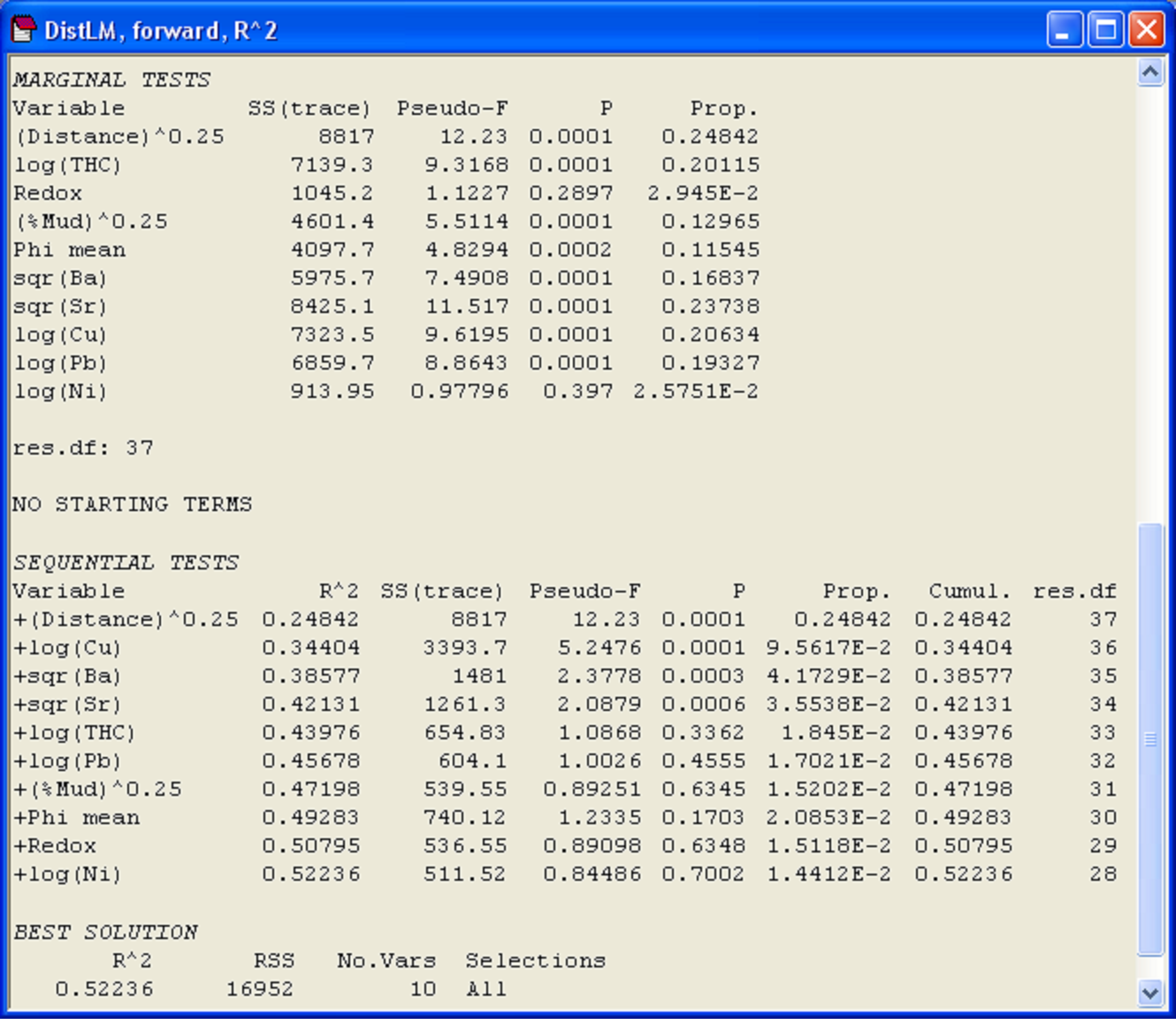
Fig. 4.12. Results of DISTLM for Ekofisk macrofauna using forward selection of transformed environmental sediment variables.
A notable aspect of the sequential tests is that after fitting the first four variables: (Distance)^(0.25), log(Cu), sqr(Ba) and sqr(Sr), the P-value associated with the conditional test to add log(THC) to the model is not statistically significant and is quite large (P = 0.336). There is probably no real further mileage to be gained, therefore, by including log(THC) or any of the other subsequently fitted terms in the model. The first four variables together explain 42.1% of the variation in community structure, and subsequent variables add very little to this (only about 1.5-2% each). Given that we had noticed earlier a very strong correlation between log(THC) and sqr(Sr), it is not surprising that the addition of log(THC) is not really worthwhile after sqr(Sr) is already in the model. Although all of the P-values for this and the subsequent conditional tests are reasonably large (P > 0.17 in all cases), the conditional P-values in forward selection do not necessarily continue to increase and, indeed, a “significant” P-value can crop up even after a large one has been encountered in the list. It turns out that little meaning can be drawn from P-values for individual terms (whether large or small) after the first large P-value has been encountered in a series of sequential tests, as the inclusion of a non-significant term in the model such as this will affect subsequent results in various unpredictable ways, depending on the degree of inter-correlations among the variables.
Based on the forward selection results, we might consider constructing and using a model with these first four chosen variables only. This is clearly a more parsimonious model than using all 10 variables. However, the forward selection procedure is not necessarily guaranteed to find the best possible model for a given number of variables. We shall therefore explore some alternative possible parsimonious models using the AIC and BIC criteria, in turn. From the resemblance matrix, choose PERMANOVA+ > DISTLM > (Predictor variables worksheet: ekevt) & (Selection Procedure •Best) & (Selection Criterion •AIC) & (Best > (Max num of best results: 10) & (Results detail: Normal) ). There is no need to do the marginal tests again, so remove the $\checkmark$ from this option.
When the ‘Best’ selection procedure is used, there are two primary sections of interest in the output. The first is entitled ‘Best result for each number of variables’ (Fig. 4.13). For example, in the present case, the best single variable for modelling the species data cloud is identified as variable 1, which is (Distance)^(0.25). The best 2-variable model, interestingly, does not include variable 1, but instead includes variables 6 and 7, corresponding to sqr(Ba) and sqr(Sr), respectively. The best 4-variable model has the variables numbered 1 and 6-8, which correspond to (Distance)^(0.25), sqr(Ba), sqr(Sr) and log(Cu). Note that the best 4-variable model is not quite the same as the 4-variable model that was found using forward selection, although these two models have values for R$^2$ that are very close. Actually, it turns out that it doesn’t matter which selection criterion you choose to use (R$^2$, adjusted R$^2$, AIC, AIC$_c$ or BIC), this first section of results in the output from a ‘Best’ selection procedure will be identical. This is because, for a given number of predictor variables, the ‘penalty’ term being used within any of these criteria will be identical, so all that will distinguish models having the same number of predictor variables will be the value of $SS _ \text{Residual}$ or, equivalently, R$^2$.
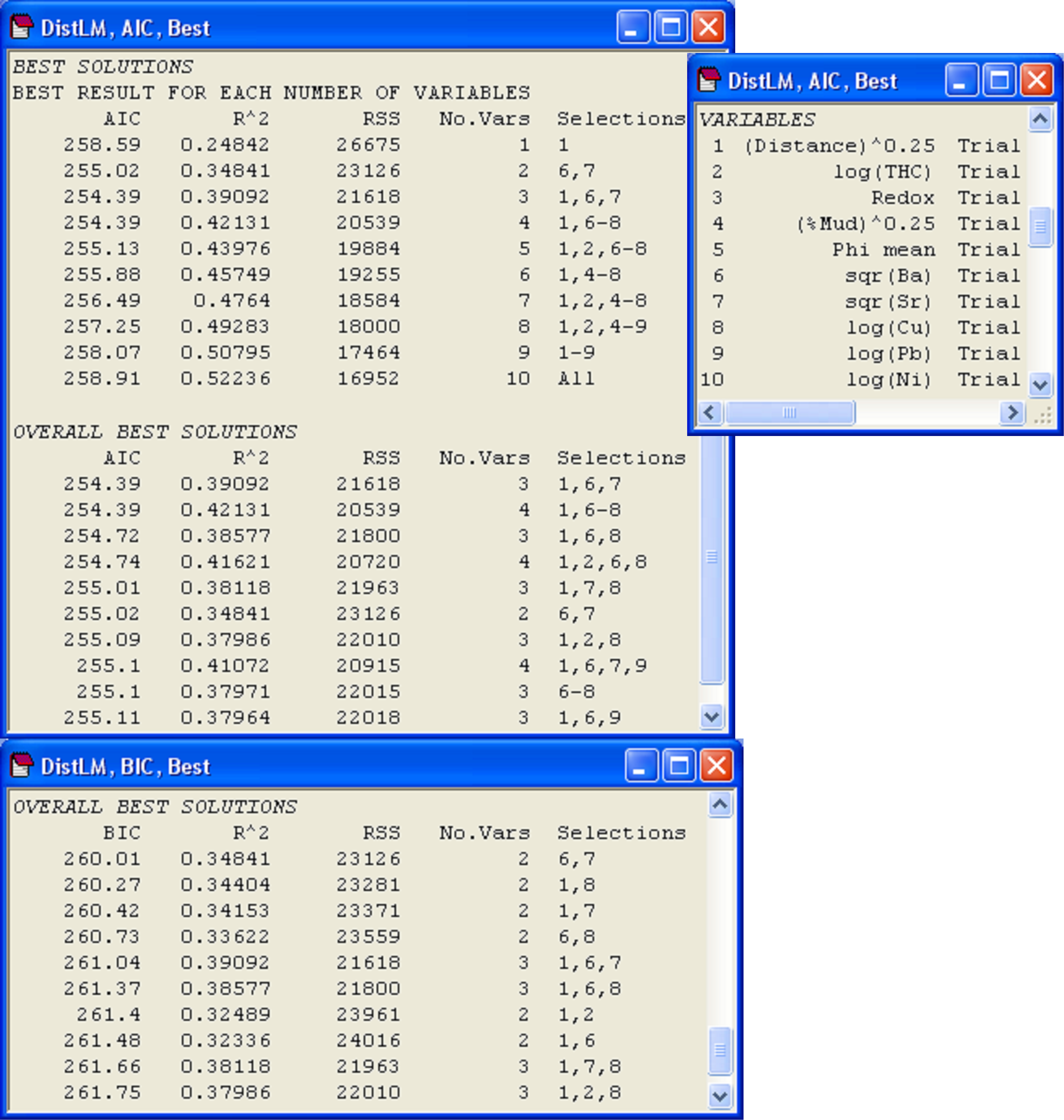
Fig. 4.13. Results of DISTLM for Ekofisk macrofauna using the ‘Best’ selection procedure on the basis of the AIC selection criterion and then (below this) on the basis of the BIC selection criterion.
The next section of results is entitled ‘Overall best solutions’, and this provides the 10 best overall models that were found using the AIC criterion (Fig. 4.13). The number of ‘best’ overall models and the amount of detail provided in the output can be changed in the DISTLM dialog. For the Ekofisk data, the model that achieved the lowest value of AIC (and therefore was the best model on the basis of this criterion) had three variables: 1, 6 and 7 (i.e., (Distance)^(0.25), sqr(Ba) and sqr(Sr) ). Another model that achieved an equally low value for AIC had 4 variables: 1, 6-8. Indeed, a rather large number of models having 3 or 4 variables achieved an AIC value that was within 1 unit of the best overall model, and even one of the 2-variable models (6, 7) was within this range. Burnham & Anderson (2002) (page 131), suggested that models having AIC values within 2 units of the best model should be examined more closely to see if they differ from the best model by 1 parameter while still having essentially the same value for the first (non-penalty) term in equation (4.6). In such cases, the larger model is not really competitive, but only appears to be “close” because it adds a parameter and is therefore within 2 units of the best model (2 $\nu$ = 2 where $\nu$ = 1), even though the fit (as measured by the first term in equation 4.6) is not genuinely improved. Generally, when a number of models produce quite similar AIC values (within 1 to 2 units of each other, as seen here), this certainly suggests that there is a reasonable amount of redundancy among the variables in X, so whichever model is eventually settled on, it is likely that a number of different combinations of predictor variables could be used inter-changeably in order to explain the observed relationship, due to these inter-correlations.
For comparison, we can also perform the ‘Best’ selection procedure using the BIC criterion (Fig. 4.13). The more “severe” nature of the BIC criterion is apparent straight away, as many of the best overall solutions contain only 2 or 3 variables, rather than 3 or 4, as were obtained using AIC. However, a few of the models listed in the top 10 using BIC coincide with those listed using AIC, including {6, 7}, {1, 6, 7}, {1, 6, 8}, {1, 7, 8} and {1, 2, 8}. To achieve a balance between the more severe BIC criterion and the more generous AIC criterion, we could output the top, say, 20 models for each and then examine a scatter-plot of the two criteria for these models. This has been done for the Ekofisk data (Fig. 4.14). An astute choice of symbols (one being hollow and larger than the other) makes it easy to identify the models that appeared in both lists. Note that from the AIC list, it is easy to calculate the BIC criterion (and vice versa), as $SS _ \text{Residual}$ (denoted ‘RSS’ in the output file) and the number of variables in the model (which is $\nu$ – 1) are provided for each model in the list.
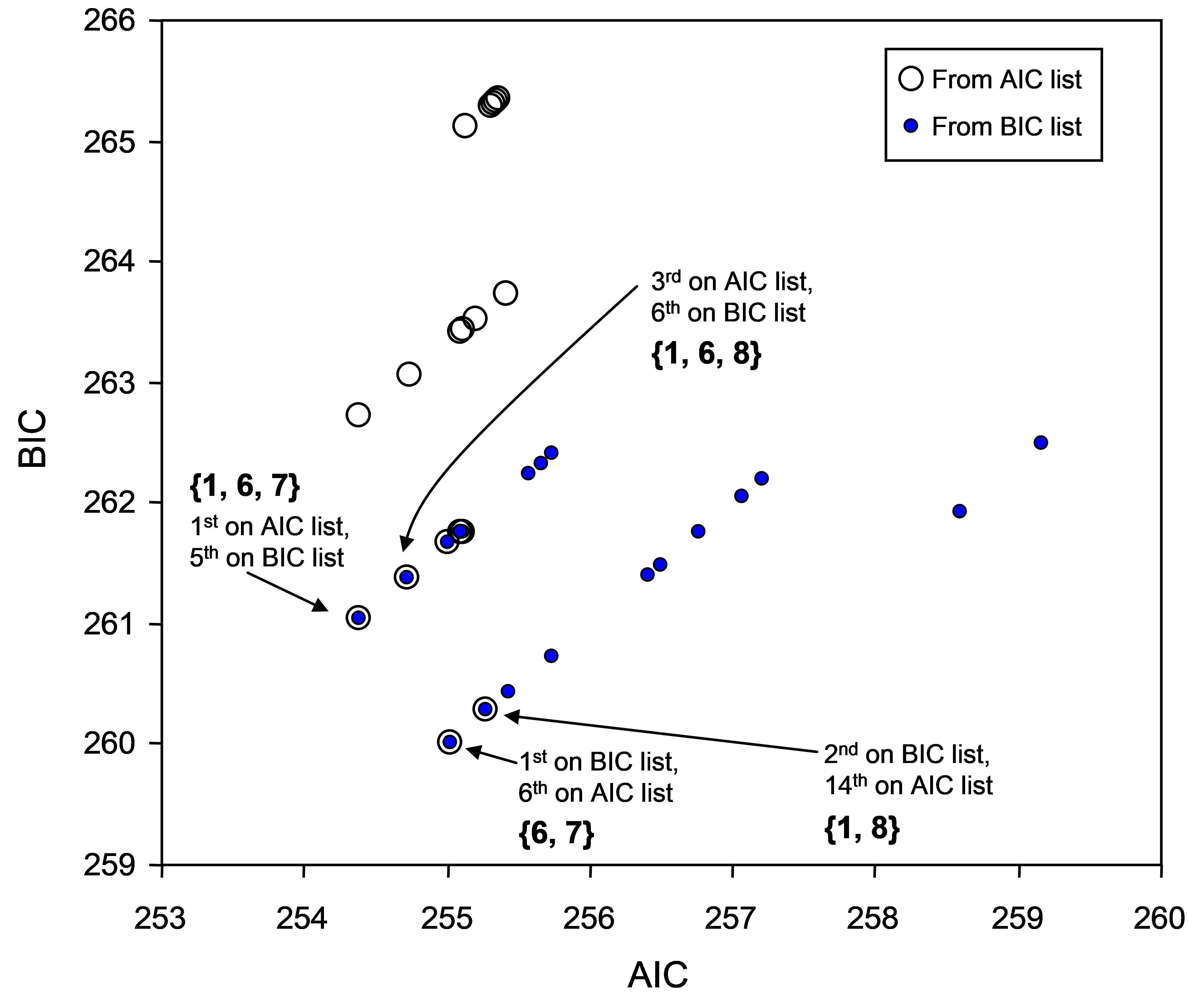 Fig. 4.14. Scatterplot of the AIC and BIC values for each of the top twenty models on the basis of either the AIC criterion or on the basis of the BIC criterion. Some of these models overlap (i.e. were chosen by both criteria).
The exact correlation between AIC and BIC for models having a given number of variables is evident in the scatter plot, as individual models occur along a series of parallel lines (Fig. 4.14). These lines correspond to models having 1 variable, 2 variables, 3 variables, and so on. In this example, most of the best models have 2, 3 or 4 variables. The greatest overlap in models that were listed in the top 20 using either the AIC or BIC criterion occurred for 3-variable models. Moreover, the plot suggests that any of the following models would probably be reasonable parsimonious choices here: {1, 6, 7}, {6, 7} or {1, 6, 8}. Balancing “severity” with “generosity”, we might choose for the time being to use the 3-variable model (bowing to AIC) which had the lowest BIC criterion, i.e., model {1, 6, 7}: (Distance)^(0.25), sqr(Ba) and sqr(Sr), which together explained nearly 40% of the variability in macrofaunal community structure. In making a choice such as this, it is important to bear in mind the caveats articulated earlier with respect to multi-collinearity and to refrain from making any direct causative inferences for these particular variables.
87 This contrasts with the use of the RELATE or BEST procedures in PRIMER, which would require normalisation prior to analysis for situations such as this.
4.11 Visualising models: dbRDA
We may wish to visualise a given model in the multivariate space of our chosen resemblance matrix. The ordination method of PCO was introduced in chapter 3 as a way of obtaining orthogonal (independent) axes in Euclidean space that would represent our data cloud, as defined by the resemblance measure chosen, in order to visualise overall patterns. PCO is achieved by doing an eigenvalue decomposition of Gower’s centred matrix G (Fig. 3.1). Such an ordination is considered to be unconstrained, because we have not used any other variables or hypotheses to draw it. Suppose now that we have a model of the relationship between our data cloud and one or more predictor variables that are contained in matrix X. We have constructed the projection matrix H, and produced the sums of squares and cross-products matrix of fitted values HGH in order to do the partitioning (Fig. 4.2). Distance-based redundancy analysis (dbRDA) is simply an ordination of the fitted values from a multivariate regression model; it is achieved by doing an eigenvalue decomposition of matrix HGH (Fig. 4.15). That is:
- Eigenvalue decomposition of matrix HGH yields eigenvalues ( $\gamma ^ 2 _ l$ , $l$ = 1, …, s) and their associated eigenvectors.
- The dbRDA axes Z (also called dbRDA “scores”) are obtained by scaling (multiplying) each of the eigenvectors by the square root of their corresponding eigenvalue.
 Fig. 4.15. Schematic diagram of distance-based redundancy analysis as a constrained ordination: an eigenvalue decomposition of the sums of squares and cross products of the fitted values from a model.
The result is a constrained ordination, because it will produce axes that must necessarily be directly and linearly related to the fitted values and, therefore, the predictor variables. If Euclidean distances are used at the outset to produce matrix D, then G = YY′ (where Y has been centered) and dbRDA is equivalent to doing a traditional RDA directly on a matrix of p response variables Y. The number of dbRDA axes that will be produced (denoted by s above and in Fig. 4.15) will be the minimum of (q, (N – 1)). If the resemblance measure used is Euclidean, then s will be the minimum of (p, q, (N – 1)). As with most ordination methods, we can draw the first two or three dbRDA axes and examine patterns among the samples seen on the plot.
A dbRDA plot can be obtained within PRIMER in one of two ways using the new PERMANOVA+ add-on: either directly for a given resemblance matrix by choosing PERMANOVA+ > dbRDA and then providing the name of a worksheet containing the predictor variables to be used (all of the variables in this worksheet that are selected will be used in this case), or by ticking the option ($\checkmark$Do dbRDA plot) in the DISTLM dialog. For the latter, the dbRDA plot will be done on the predictor variables selected by the DISTLM routine, as obtained using the selection procedure and selection criterion chosen by the user.
Initial interest lies in determining the adequacy of the plot. More specifically, how much of the fitted model variation is captured by the first two (or three) dbRDA axes? As for other eigenvalue decomposition techniques (such as PCA or PCO), the eigenvalues88 are ordered from largest to smallest and yield information regarding the variation explained by each orthogonal (independent) dbRDA axis. The sum of the eigenvalues from dbRDA is equal to the total explained variation in the fitted model, that is: $\sum \gamma^2 _ l = tr ( \text{\bf HGH} ) = SS _ \text{Regression}$. So, the percentage of the fitted model’s variation that is explained by the $l$th dbRDA axis is (100 × $ \gamma^2 _ l / \sum \gamma^2 _ l $ ). As with PCO or PCA, we consider that if the percentage of the fitted variation that is explained by the diagram exceeds ~ 70%, then the plot is likely to capture most of the salient patterns in the fitted model.
Another relevant conceptual point regarding dbRDA is that there is an important difference between the percentage of the fitted variation explained by a given axis, as opposed to the percentage of the total variation explained by that axis. The latter is calculated as (100 × $ \gamma^2 _ l / tr ( \text{\bf G} ) $ or (100 × $ \gamma^2 _ l / \sum \lambda _ i $), where $\sum \lambda _ i $ is the sum of PCO eigenvalues. The dbRDA axis might be great at showing variation according to the fitted model, but if the model itself only explains a paltry amount of the total variation in the first place, then the dbRDA axis may be of little overall relevance in the multivariate system as a whole. It is therefore quite important to consider the percentage of explained variation for each dbRDA axis out of the fitted and out of the total variation. Another way of thinking about this is to compare the patterns seen in the dbRDA plot with the patterns seen in the unconstrained PCO plot. If the patterns are similar, then this indicates that the model is a pretty good one and captures much of what can be seen overall in the multivariate data cloud. Such cases should also generally correspond to situations where the R$^2$ for the model ($ SS _ \text{ Regression } / SS_ \text{ Total } = \sum \gamma^2 _ l / \sum \lambda _ i $) is fairly large. In contrast, if the pattern in the dbRDA and the PCO are very different, then there are probably other factors that are not included in the model which are important in driving overall patterns of variation.
88 The eigenvalues from a redundancy analysis are sometimes called “canonical eigenvalues”, as in chapter 11 in Legendre & Legendre (1998) .
4.12 Vector overlays in dbRDA
Something which certainly should come as no surprise is to see the X variables playing an important role in driving the variation along dbRDA axes. Of course, the X variables must feature strongly here, because it is from these that the fitted variation is derived! To characterise the dbRDA axes, it is useful to determine the strength and direction of the relationship between individual X variables and these axes. A common method for visualising these relationships is to examine vector overlays on the ordination diagram, with one vector for each predictor variable. The positions and directions of appropriate vectors can be obtained by calculating the multiple partial correlations between each of the X variables and the dbRDA axis scores. These vectors can be interpreted as the effect of a given predictor variable on the construction of the constrained ordination picture – the longer the vector, the bigger the effect that variable has had in the construction of the dbRDA axes being viewed. If the ordination being viewed explains a large proportion of the variation in the fitted model (and we would hope that this is indeed generally true), then these vectors are also representative of the strength and direction of influence of individual X variables in the model itself. Note that these vectors show the strength of the relationships between each predictor variable and the dbRDA axes, given that it is fitted simultaneously with the other X variables in the model. In other words, the calculation of the correlation between each X variable and each dbRDA axis is conditional upon (i.e. takes into account) all of the other X variables in the worksheet.
Although the above vector overlay is shown by default in the dbRDA ordination graphic, there are other kinds of potentially informative vector overlays. For example, one might choose to plot the simple Pearson (or Spearman) correlations of the X variables with the dbRDA axes, as was shown for PCO plots in the section Vector overlays in chapter 3. Note, however, that each of these vectors is drawn individually, ignoring the other variables in the worksheet89. In PRIMER, there are therefore three different kinds of vector overlays offered for dbRDA plots as part of the PERMANOVA+ add-on. These are obtained as follows from within the ‘Configuration Plot’ dialog90 (presuming for the moment that the predictor variables that gave rise to the model are located in a worksheet named X):
-
Default dbRDA vector overlay, corresponding to multiple partial correlations of the (centred) X variables with the dbRDA axes: choose (Vectors: •Base variables). These vectors are identical to those that are obtained using the choice (Vectors: •Worksheet variables: X > Correlation type: Multiple).
-
Pearson simple linear correlations of individual X variables with the dbRDA axes: choose (Vectors: •Worksheet variables: X > Correlation type: Pearson)
-
Spearman simple rank correlations of the X variables with the dbRDA axes: choose (Vectors: •Worksheet variables: X > Correlation type: Spearman)
Of course, some other variables (and not just the predictor variables that gave rise to the dbRDA axes) can also be superimposed on the dbRDA ordination diagram using this general vector overlay tool. Bubble plots (see p. 83 in chapter 7 of Clarke & Gorley (2006) ) can also be useful to visualise the relative values of an individual variable among sample points in a dbRDA ordination.
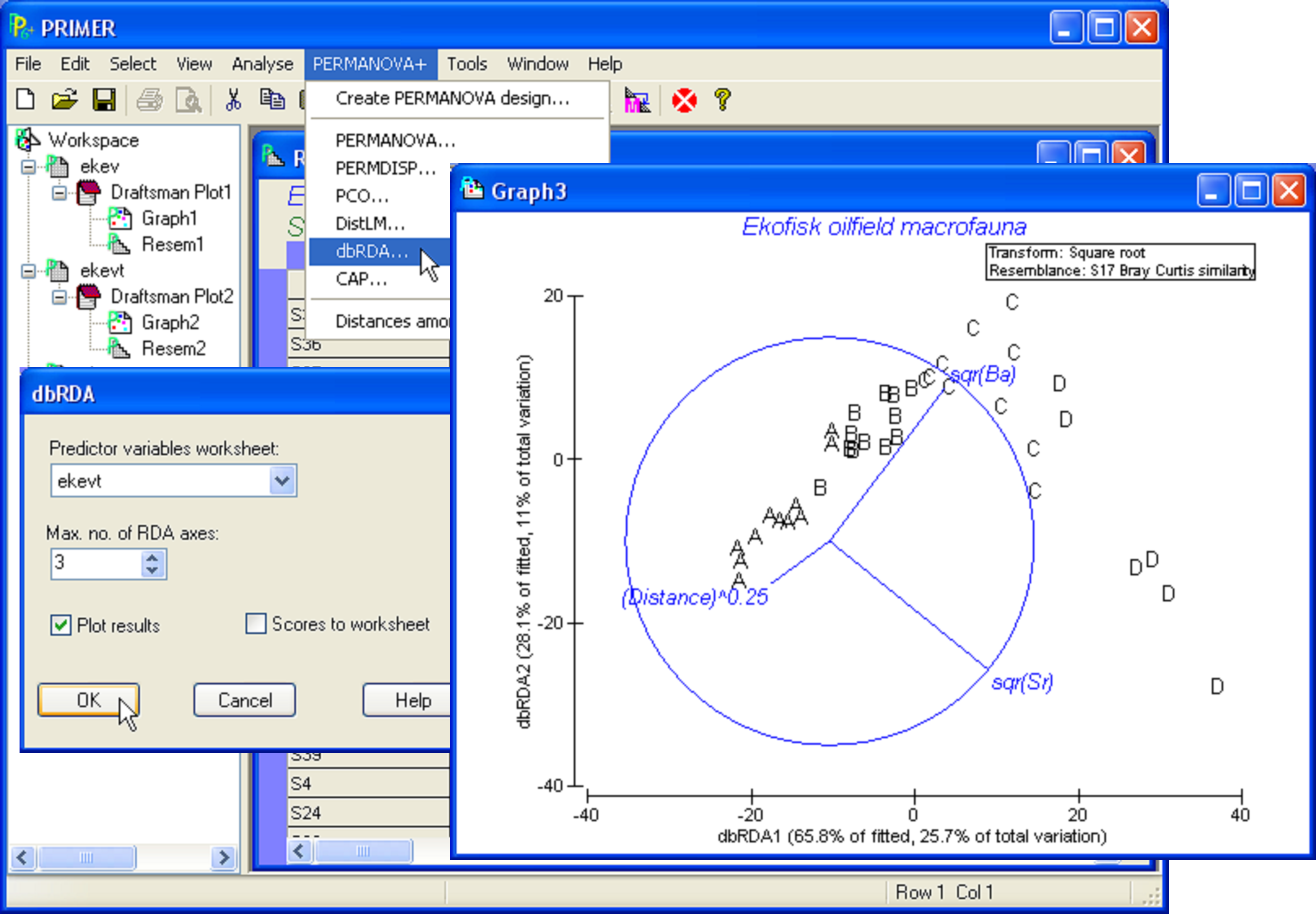
Fig. 4.16. dbRDA of the Ekofisk data from the parsimonious model with three environmental variables.
Clearly, the type of vectors to plot is up to the user and depends on the type of information being sought. When publishing a dbRDA plot as part of a study, it is important to give information about the variation explained by the axes (out of the fitted and out of the total variation) and also to indicate which type of vector overlays are being used, if any are displayed. Of course, all of the other graphical options and tools available from within PRIMER are also able to be used in dbRDA plots, including 3-dimensional representation, spin, options for symbols and labels, fonts, colours, and so on. See Clarke & Gorley (2006) for more details.
89 Although ter Braak (1990) suggested that individual Pearson correlations (ignoring other X variables) are most informative, Rencher ( Rencher (1988) , Rencher (1995) ) disagrees, stating that the multivariate nature of these inter-relationships is ignored by using raw correlations, which show only univariate relationships. Both types of vector overlay are available within the PERMANOVA+ add-on.
90 The ‘Configuration Plot’ dialog is obtained for any plot by choosing Graph > Special.
4.13 dbRDA plot for Ekofisk
Let us examine the constrained dbRDA ordination for the parsimonious model obtained earlier using DISTLM on the Ekofisk data. The parsimonious model we had settled on included three predictor variables: (Distance)^(0.25), sqr(Ba) and sqr(Sr). Go to the ekevt worksheet, highlight and then select these three variables by choosing Select > Highlighted. Now return to the resemblance matrix based on the macrofaunal data and choose PERMANOVA+ > dbRDA > (Predictor variable worksheet: ekevt) & (Max. no. of dbRDA axes: 3) & ($\checkmark$Plot results). The resulting pattern among the samples (Fig. 4.16) suggests that there are effectively two gradients (forming sort of an upside-down “V” shape) in the community structure of the macrofauna that can be modeled by these environmental variables. The first largely distinguishes among groups A, B, C and D and is (not surprisingly) driven largely by distance from the oil platform, as well as the concentrations of Ba in the sediments. The second gradient identifies variability among the sites within group D that are close to the oil platform (< 250 m). These differences are apparently mostly driven by differences in the concentrations of Sr in the sediments. We shouldn’t forget, however, that sqr(Sr) had a very strong relationship (r = 0.92) with log(THC), so the modeled variation in community structure among these samples near the platform could just as easily be due to variation in total hydrocarbons as to strontium concentrations (or to the combined effects of both, or to some other unmeasured variables)91.
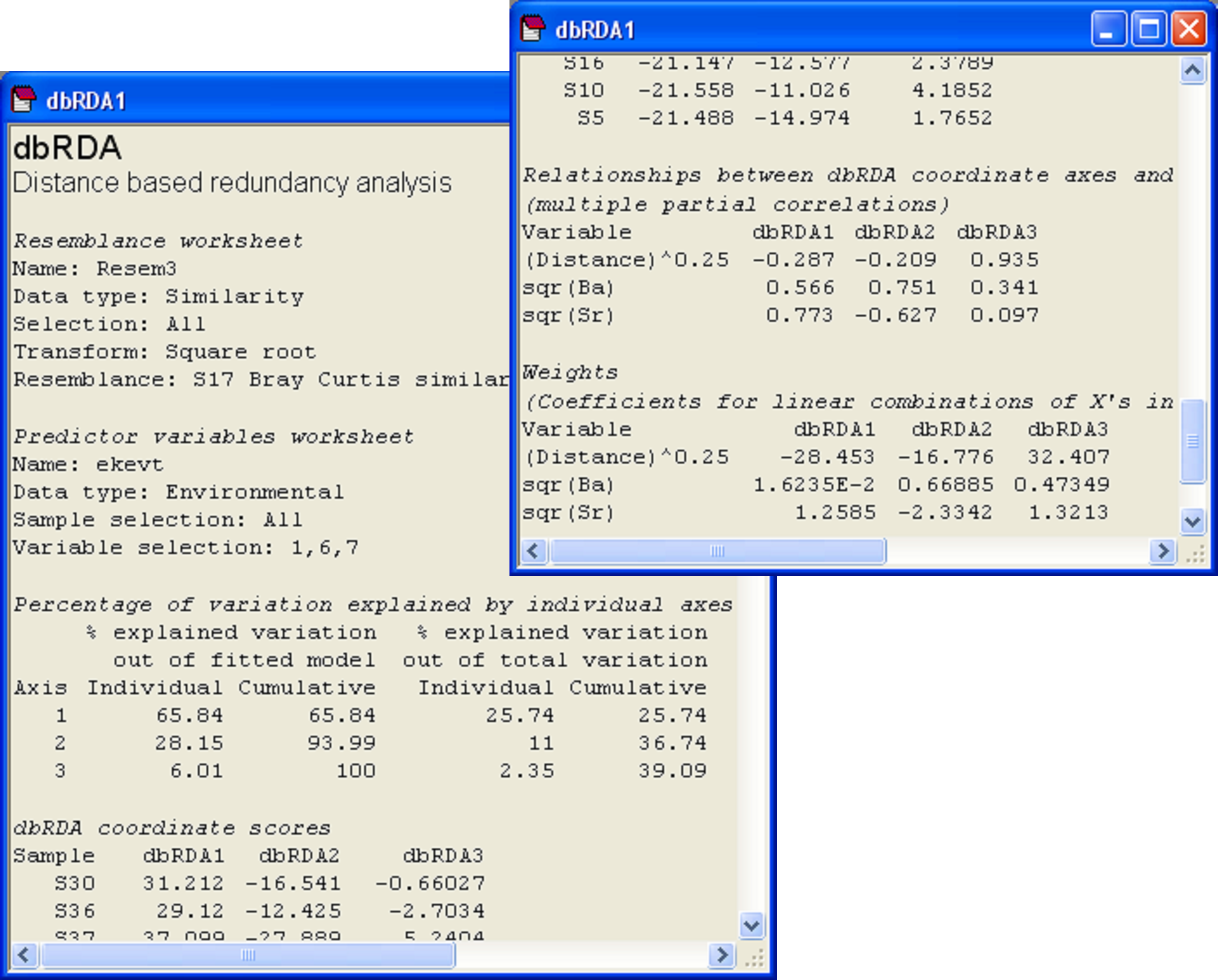
Fig. 4.17. Output file from dbRDA of the Ekofisk macrofauna vs three environmental variables.
Other output provided from running the dbRDA routine shows more information about the dbRDA axes (Fig. 4.17). First, we are given information that will help to assess the adequacy of the ordination plot. The first two columns in the section entitled ‘Percentage of variation explained by individual axes’ relate to the percentage explained out of the fitted model (i.e., out of tr(HGH) or SS$_ \text{Regression} $). The next two columns in this section relate to the percentage explained out of the total variation in the resemblance matrix (i.e., out of tr(G) or SS$_ \text{Total} $). In the present case, the first two dbRDA axes explain 94.0% of the fitted variation, and this is about 36.7% of the total variation in the resemblance matrix. So, we can rest assured that these two dbRDA axes are capturing pretty much everything we should wish to know about the fitted model, although there is sill quite a lot of residual variation in the original data matrix which is not captured in this diagram. Note that there are three dbRDA axes as s = min( q, (N – 1) ) = min( 3, 38 ) = 3. All of the dbRDA axes together explain 100% of the fitted variation. Taken together, they also explain 39.1% of the total variation. This is equal to 100 × R$^2$ from the DISTLM model for these three variables (Fig. 4.13).
Another way to check the overall utility and adequacy of the model as it is shown in the constrained dbRDA plot is to compare it with an unconstrained PCO plot of the same data. If the patterns of sample points in the two plots are similar, then this indicates that the dbRDA (and by implication, the model) is doing a good job of finding and explaining the most salient patterns of variation across the data cloud as a whole. If, on the other hand, these two plots are quite different, then, although it does not mean the model is useless, it does indicate that there are likely to be some other structuring forces out there which were not measured or included in the model. The PCO plot of the Ekofisk data shows a remarkably similar pattern to the dbRDA plot (Fig. 4.18), indicating that this three-variable model is indeed capturing the most salient overall patterns of variability. Although there is still quite a lot of unexplained variation (even the first two PCO axes explain only 43.1% of the total), these are the axes of greatest variation through the data cloud defined by the resemblance measure chosen and thus the environmental drivers used in the model (and variables correlated with them) are very likely to be the most important drivers of differences in macrofaunal community structure among these samples.
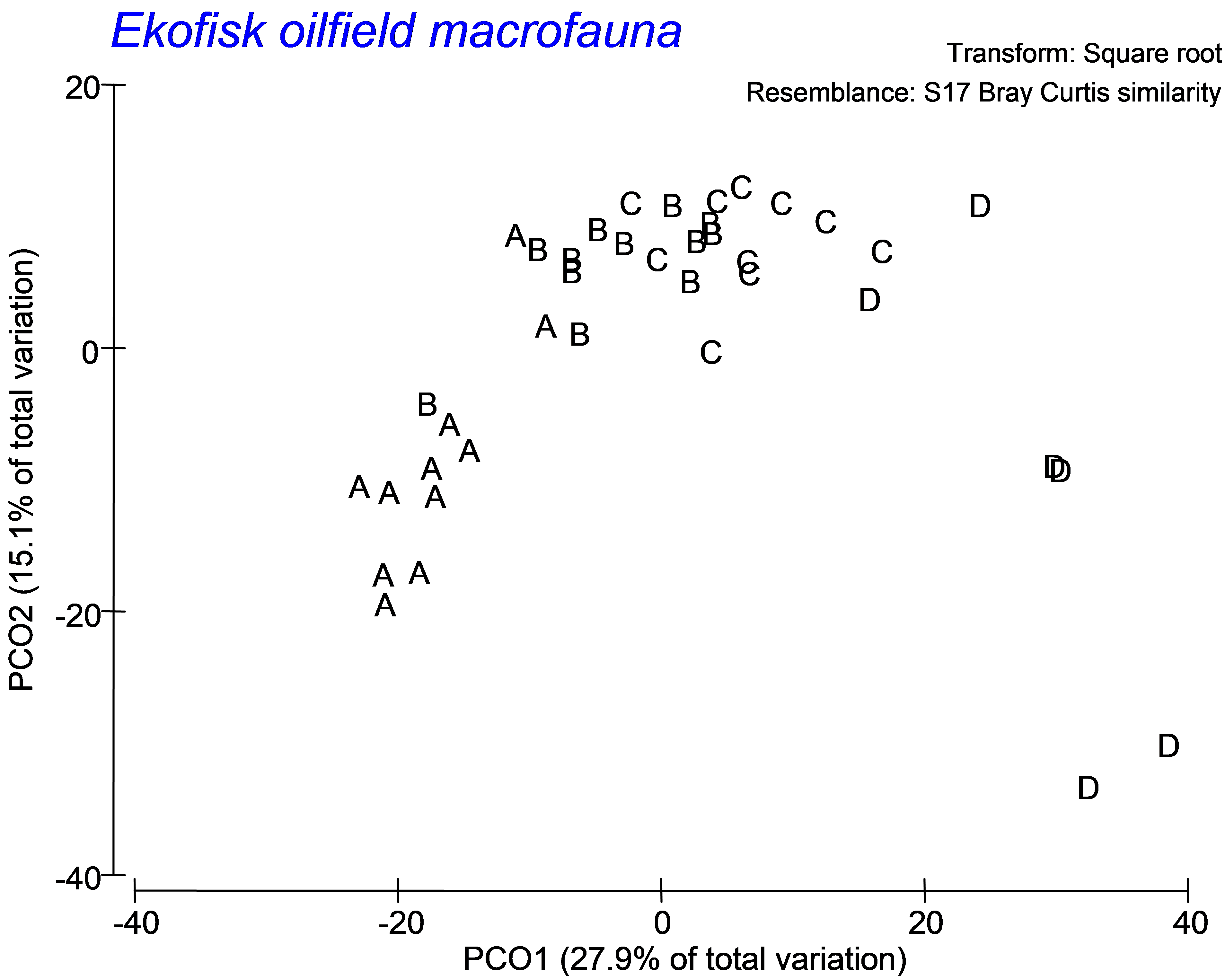 Fig. 4.18. PCO of the Ekofisk macrofauna.
The next portion of the output file provides the dbRDA coordinate scores (Fig. 4.17). These are the positions of the samples along the dbRDA axes and they can also be output into a separate worksheet by ticking the ($\checkmark$Scores to worksheet) option in the dbRDA dialog. Next, the output file provides information regarding the vector overlay positions of each variable along each axis (Fig. 4.17). Specifically, under the heading ‘Relationships between dbRDA coordinate axes and orthonormal X variables’, are given the values of the multiple partial correlations; these are the values that are plotted in the default dbRDA vector overlay.
The last portion of the output from dbRDA shows the relative importance of each X variable in the formation of the dbRDA axes (Fig. 4.17). These are entitled ‘Weights’ and subtitled ‘(Coefficients for linear combinations of X's in the formation of dbRDA coordinates)’. Recall that the dbRDA axes are linear combinations of the fitted values and that these, in turn, are linear combinations of the original X variables. Thus, we can obtain the direct conditional relationships of individual X variables in the formation of each dbRDA axis by multiplying these two sets of linear combinations together. The resulting weights given here are identical to the standardised partial regression coefficients that would be obtained by regressing each of the dbRDA axes scores (Z) directly onto the matrix of normalised explanatory variables X92.
91 Quite similar roles for Ba and THC as those described here were outlined for this data set by Clarke & Gorley (2006) (p. 84, chapter 7) from examining bubble plots of these environmental variables on the species MDS plot, although no formal modeling of these relationships was done in that purely non-parametric setting.
92 If a Euclidean distance matrix was used as the basis of the dbRDA analysis, these weights correspond precisely to the matrix called C in equation 11.14 on p. 585 of Legendre & Legendre (1998) .
4.14 Analysing variables in sets (Thau lagoon bacteria)
In some situations, it is useful to be able to partition variability in the data cloud according to sets of predictor variables, rather than treating each variable individually. For example, Borcard, Legendre & Drapeau (1992) discussed the partitioning of variation in multivariate species data among two sets of variables: a set of environmental variables and a set of spatial variables (such as latitude and longitude, arbitrary spatial coordinates, or polynomial functions of these). They considered that analyses of the relationship between species data and environmental variables should include a consideration of the intrinsic spatial structuring caused simply by the relative geographic distances among samples at a given scale. One might expect, for example, that samples close together would be more similar than those further apart. By analysing the data in sets, one can explicitly examine the proportion of variation in the species data that is explained by the environmental variables over and above the amount explained by the spatial variables alone.
DISTLM can treat variables either individually or in sets. To identify sets of variables, one needs to first define an indicator which will identify the set that a particular predictor variable belongs to. Recall that an indicator in PRIMER identifies groups of variables the same way that a factor identifies groups of samples (see chapter 2 in Clarke & Gorley (2006) ).
As an example, we shall analyse a data set on the responses of heterotrophic bacteria grown in different media (labeled ‘Ma’ and ‘Bna’) to sets of environmental and spatial variables obtained from each of 20 sites in the Thau lagoon ( Amanieu, Legendre, Troussellier et al. (1989) ) provided by Legendre & Legendre (1998) (p. 529). Data on the bacteria are located in the file thbac.pri, and the associated environmental and spatial variables are located in the file thevsp.pri, both in the ‘Thau’ folder of the ‘Examples add-on’ directory. For the bacteria, the variable Bna is the concentration of colony-forming units of aerobic heterotrophs growing on bioMérieux nutrient agar (low salinity) and Ma is the concentration growing on marine agar. The environmental variables are NH4 (ammonium in the water column, in $\mu$mol per litre), Phaeo.a (phaeopigments from degraded chlorophyll a, in $\mu$g per litre) and Prod (bacterial production, determined by incorporation of titrated thymidine in bacterial DNA, in nmol per litre per day). Each of these environmental variables and also the bacteria concentrations have already been transformed using ln(X+1). The spatial variables (named X and Y) are the positions of the samples in terms of geographic coordinates according to an arbitrary grid, and have been centred on their means. The spatial variable X2 is the square of X and is included as another spatial predictor variable of potential importance.
Open up both of these data files in PRIMER. Focusing first on the sheet containing environmental and spatial variables, choose Edit > Indicators and an indicator called (rather uncreatively) ‘Indicators’ will be shown that identifies which set (environmental or spatial, denoted by ‘Env’ or ‘Geo’, respectively) each of these predictor variables belongs to (Fig. 4.19). Indicators, like factors, can either be created from within PRIMER, or they can be brought into PRIMER along with the data file. Next, it is wise to examine a draftsman plot to see the distributions of these variables and the relationships among them, prior to fitting the model. Whether we fit the predictor variables alone or in sets, we do need to satisfy ourselves that their distributions are reasonable and check for high collinearity, removing any clearly redundant variables if necessary. For these data (Fig. 4.19), it is interesting to note that the scatterplot of the spatial variables X and Y effectively shows a map of the spatial positions of the samples. Furthermore, it is no surprise to see that X2 has a perfect quadratic relationship with X. For the rest, all seems well and we are ready to proceed.
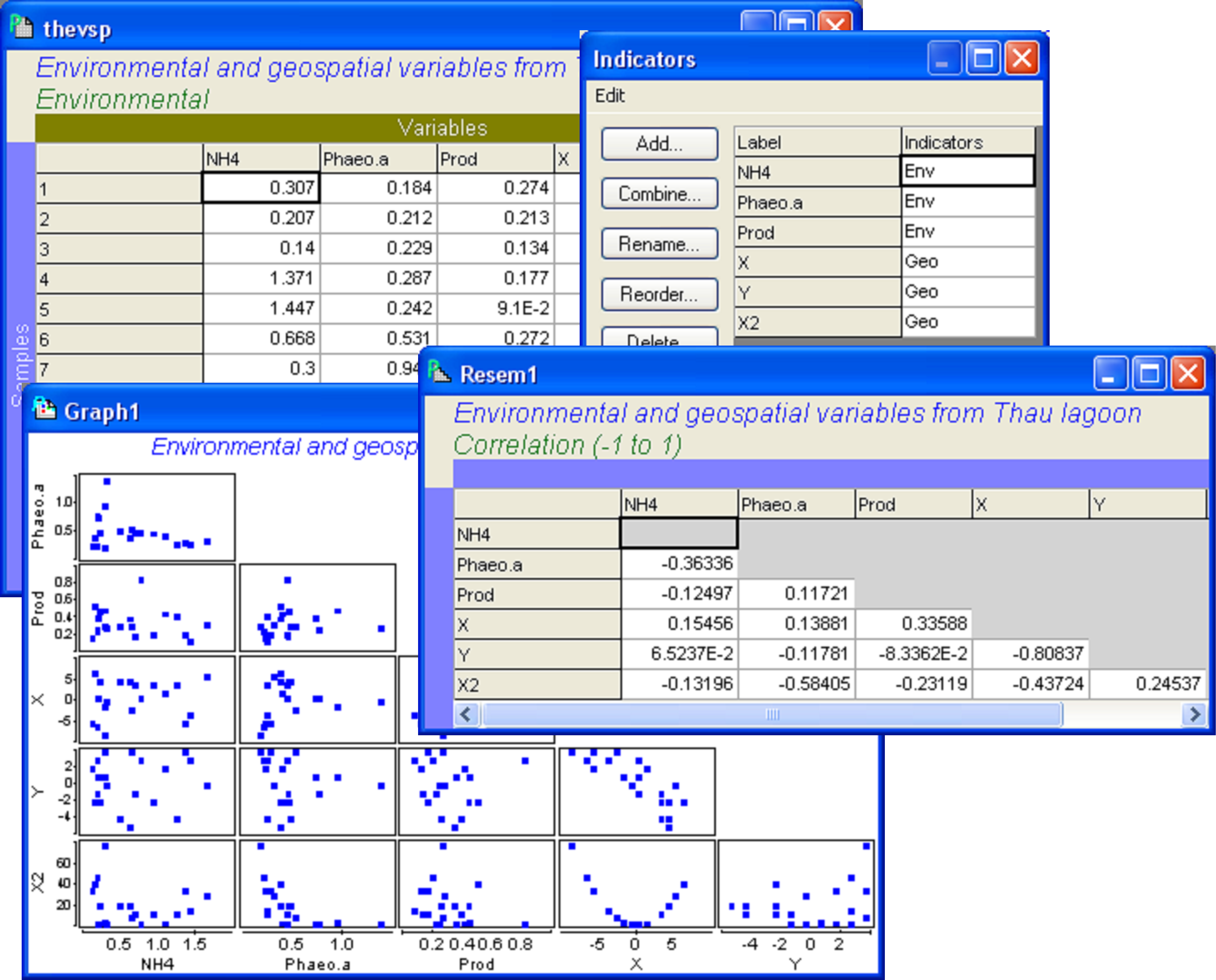
Fig. 4.19. Diagnostics examining predictor variables from the Thau lagoon.
The response variables, in this case, are concentrations of bacteria that contain no zeros and (after the log-transformation, which has already been done for these data) are quite well-behaved in their distributions (i.e., show fairly equal scatter throughout their range and are not heavily skewed). Thus, we can quite reasonably consider doing an analysis on the basis of the Euclidean distance measure. The variables are also in the same units of measurement and occur on similar scales, so no preliminary normalisation is needed here. Although normalisation of predictor variables is never required in DISTLM (and would make no difference to the results in any event), it is important to consider, when calculating Euclidean distances on the basis of a set of response variables, whether or not a prior normalisation is appropriate. For this, the usual considerations (such as the units of the variables and their relative scales) apply.
Calculate a Euclidean distance matrix from the thbac data sheet and then choose PERMANOVA+ > DISTLM > (Predictor variables worksheet: thevsp) & ($\checkmark$Group variables (indicator): Indicators) & (Selection Procedure •All specified) & (Selection Criterion •R^2) & (Num. permutations: 9999) & ($\checkmark$Do marginal tests), as shown in Fig. 4.20. Before clicking the ‘OK’ button, check out the order in which these sets of variables will be fitted by clicking on the ‘Select variables/groups…’ button. The order shown will be the order in which these groups were provided in the data file. In our case, however, it makes sense specifically to fit the ‘Geo’ set first, followed by the ‘Env’ set, as we are interested in testing the hypothesis of there being no relationship between the bacteria concentrations and the environmental variables, given the spatial variables. This can be done by highlighting Geo appearing inside the ‘Available:’ column and then clicking on the upward arrow to move it up to first in the list (Fig. 4.20).
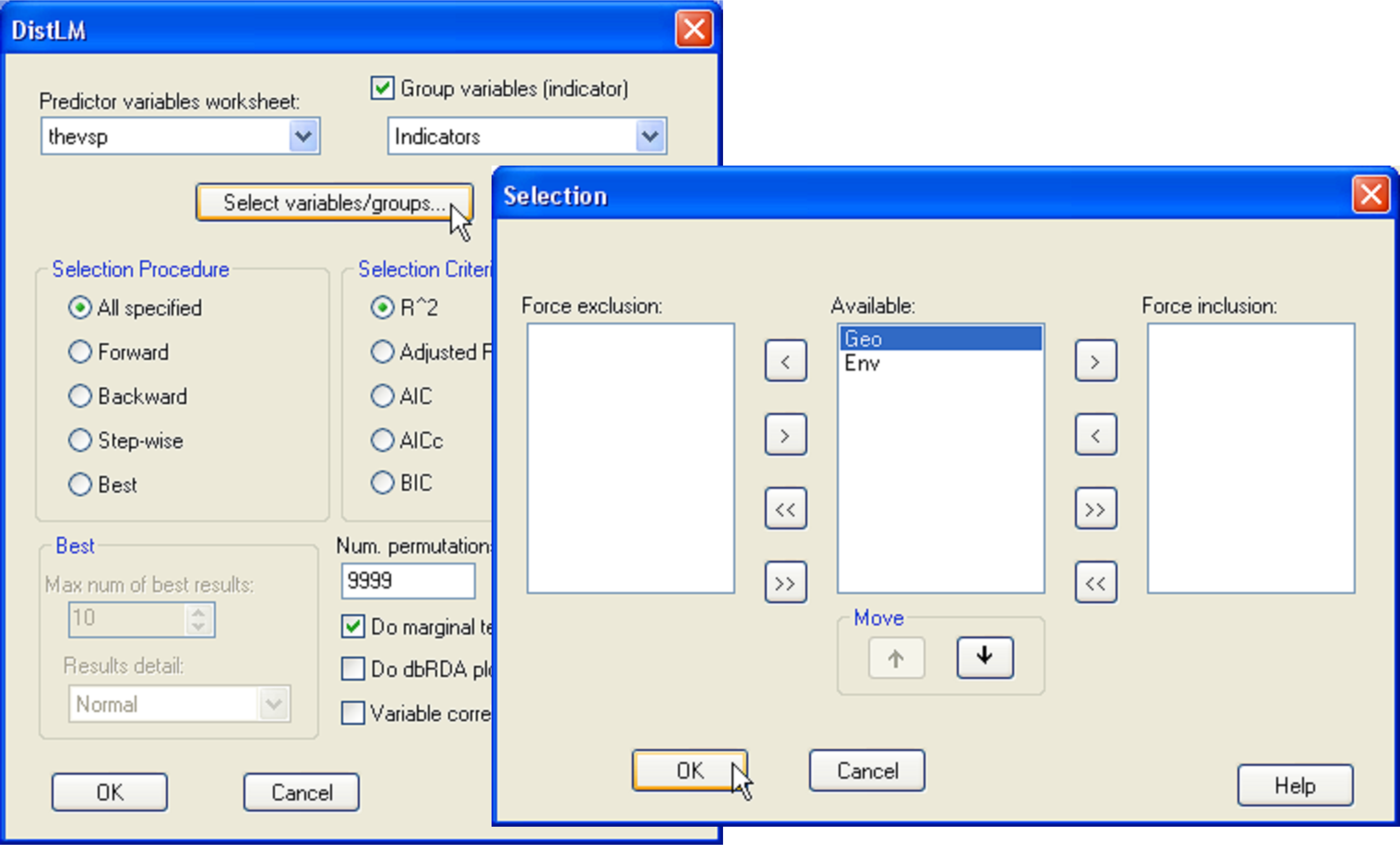 Fig. 4.20. DISTLM dialog for fitting sets of predictor variables in a particular order.
The file of results from this analysis is shown in Fig. 4.21. We can see that the three spatial variables alone accounted for 36.4% of the variation in the bacteria concentrations, while the environmental variables accounted for 45.0%. However, after fitting the spatial variables, the environmental variables explained an additional 18.5%, resulting in a total explained variation of 55%. This additional amount was not statistically significant, however, according to the sequential test (P = 0.16).
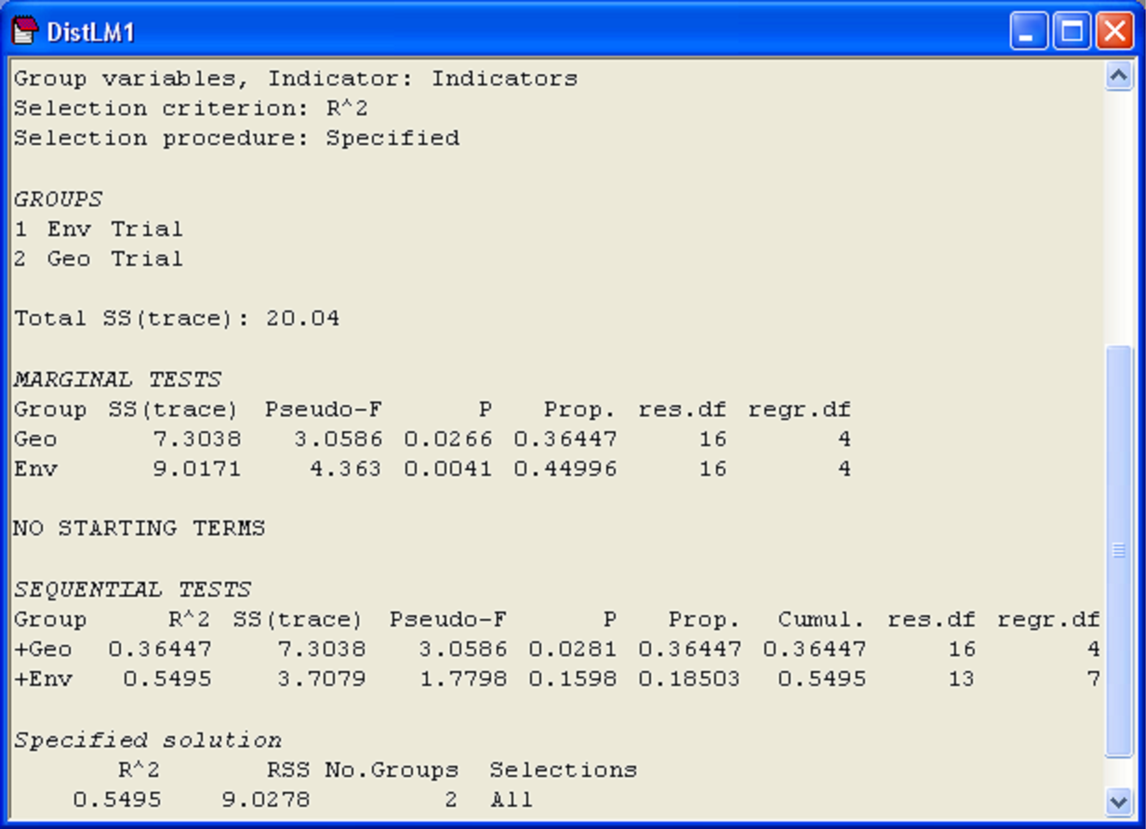 Fig. 4.21. Results of DISTLM fitting sets of predictor variables to bacteria concentrations from Thau lagoon.
Partitioning of multivariate data described by a resemblance matrix of choice in response to multiple sets of variables (as in Anderson & Gribble (1998) , for example, who partitioned temporal, spatial and environmental components) can be done in this manner, and the degree of overlap between individual sets can be readily determined by changing the order of fit of the variables, as desired. Keep in mind, however, that sets having different numbers of predictor variables will naturally have a different capability when it comes to explaining variation – a set with one variable would be expected naturally to explain less than a set with 5 variables, simply because it has fewer degrees of freedom. We have chosen in this example to use the simple R$^2$ criterion (both sets had 3 variables, so the percentage of variation explained could be directly compared), but an adjusted R$^2$, AIC, AIC$_c$ or BIC criterion could also be used, and these would (each in their own way) take into account different numbers of variables in the different sets93. Such an approach is directly analogous to examining components of variation derived from mean squares, rather than just looking at the raw partitioning of the sums of squares when comparing the relative importance of different sources of variation in a PERMANOVA model. In this example, we also had a specific hypothesis which dictated the order of the fit (the ‘Geo’ set first, followed by the ‘Env’ set), but in other situations, a different selection procedure (i.e., forward, backward, step-wise, best) might be more appropriate for the hypotheses or goals of the study.
93 Peres-Neto, Legendre, Dray et al. (2006) discussed the use of an adjusted R$^2$ criterion to perform a partitioning of multivariate response data in RDA and CCA models and to allow comparison of the sizes of portions explained by different sets of predictor variables.
4.15 Categorical predictor variables (Oribatid mites)
Sometimes the predictor variables of interest are not quantitative, continuous variables, but rather consist of categories or groups, called categorical or nominal variables. There are also situations where we have mixtures of variable types that we want to include in a single DISTLM analysis. For example, we might want to consider a single model that includes temperature and salinity (continuous and quantitative) but which also includes a categorical variable, habitat, that might be recorded for each sample as one out of a number of different types: sand, coral, rock, seagrass, etc. How can we analyse categorical predictor variables using DISTLM?
As an example, we will consider an analysis of environmental control and spatial structure in an oribatid mite community, described by Borcard, Legendre & Drapeau (1992) and Borcard & Legendre (1994) . These data come from a site adjacent to a small Laurentide lake, Lake Geai, at the Station de Biologie des Laurentides in Quebec, Canada. The species (response) data (in the file ormites.pri in the ‘OrbMit’ folder of the ‘Examples add-on’ directory) consist of counts of abundances for each of p = 35 species of oribatid mites from each of N = 70 sites. The file orenvgeo.pri (in the same folder) contains a number of predictor variables associated with each of the sites. Some of these are spatial variables and correspond to the geographic coordinates of each sample on a grid measured in metres (‘x’, ‘y’) and up to third-order polynomial functions of these (‘x2’, ‘xy’, ‘y2’, etc.). The others are environmental variables, which include two quantitative variables:
-
Substratum density (‘Substr.dens’), measured in grams per litre of dry uncompressed matter, and
-
Water content of the substratum (‘H20.cont’), measured in grams per litre, and three categorical (nominal) variables:
-
Substrate (7 categories: Sphagnum groups 1-4, litter, bare peat, interfaces),
-
Shrubs (3 categories: no shrubs, few shrubs, many shrubs), and
-
Microtopography (2 categories: blanket (flat) and hummock (raised))
The nominal variable ‘Shrubs’ is actually ordinal or semi-quantitative, so the simple rank order values of ‘1’, ‘2’ and ‘3’ in a single column could also be used here to treat this as a single (1 df) continuous quantitative predictor variable. However, we shall treat it as a nominal variable here to be consistent with the way this variable was treated by Borcard, Legendre & Drapeau (1992) and Borcard & Legendre (1994) .
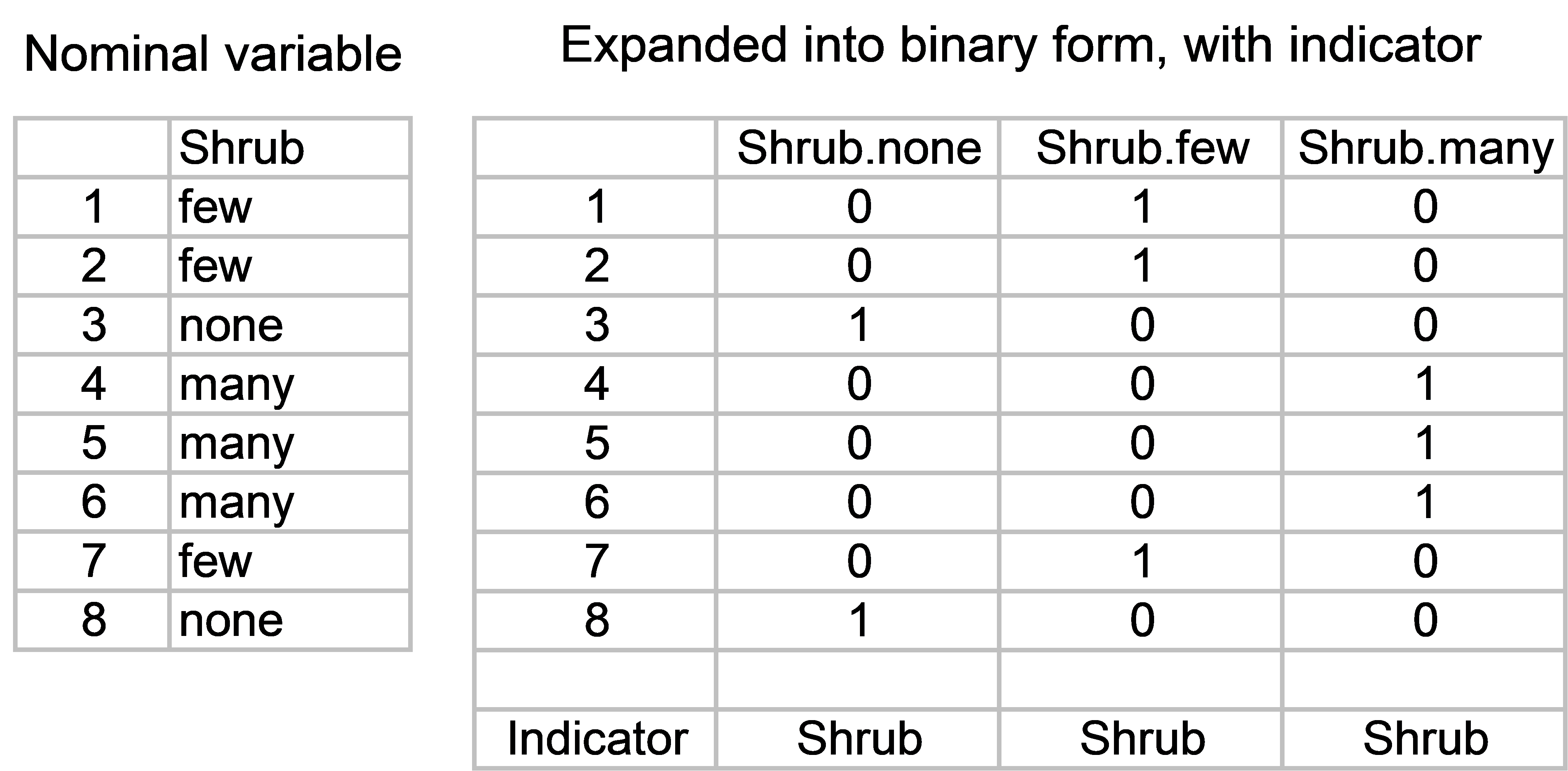
Fig. 4.22. Example of a categorical (nominal) variable and its expanded binary form.
To start with, we need to expand each categorical variable of interest into a set of “on/off” or binary variables (e.g., Fig. 4.22). For each categorical variable, there will be as many binary variables as there are categories. The binary variables will take a value of ‘1’ for samples where that category occurs, and zero (‘0’) elsewhere. Once this has been done, the binary variables associated with a particular nominal variable need to be specified as a set, using an indicator in PRIMER (see the previous section on setting up indicators to analyse sets of variables). For example, the seven “on/off” variables that “code” for each of the seven substrate categories are identified (by having a common name for the indicator) as belonging to the ‘Substrate’ set. If there are also quantitative variables to be analysed as part of the same predictor variable worksheet, then each of these can simply be specified in the indicator as belonging to its own “set”. The environmental data, with the categorical variables already expressed as binaries and identified in sets using the indicator called ‘Type’, are located in the file orenvgeo.pri (Fig. 4.23).
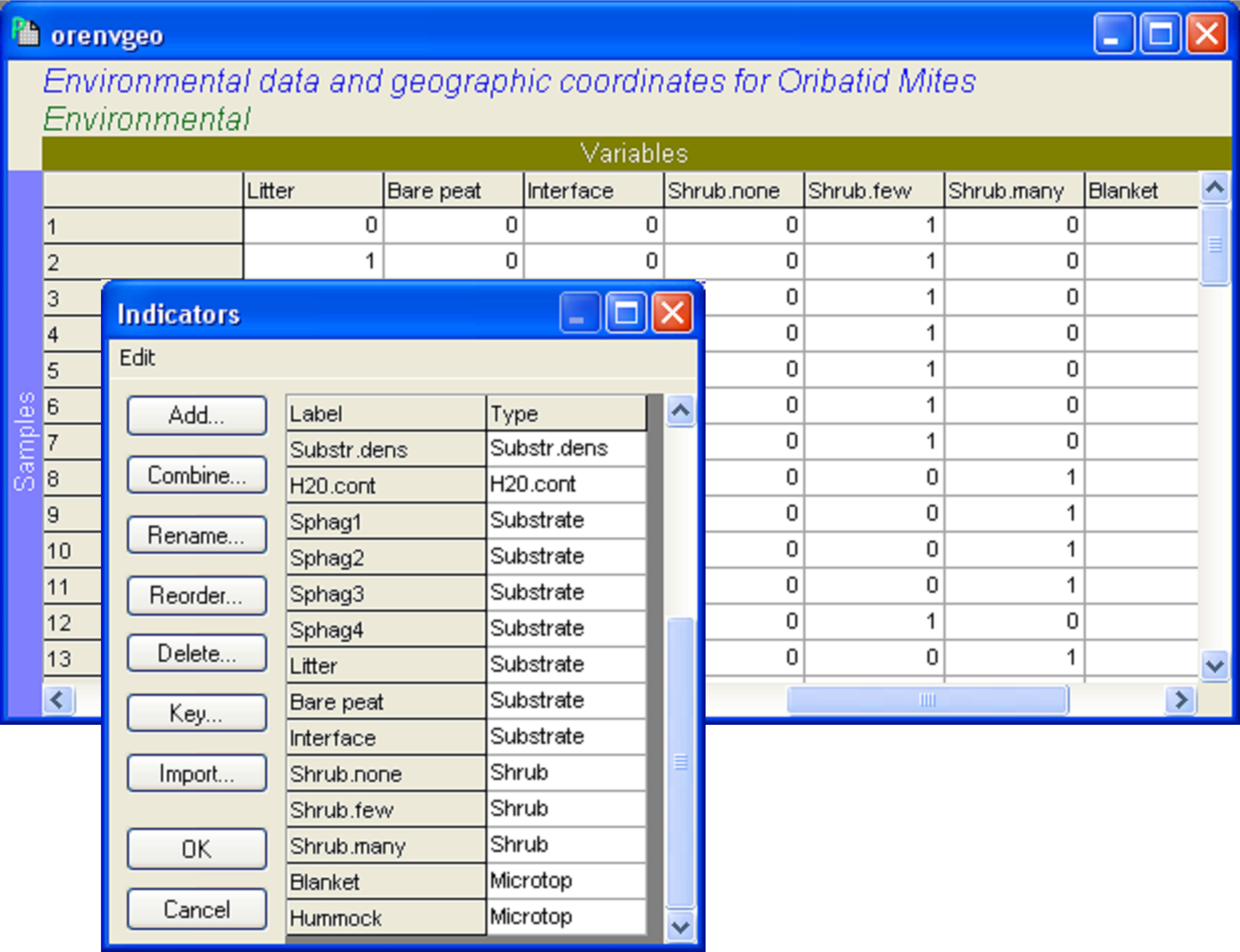
Fig. 4.23. Environmental variables in binary form and their indicator (‘Type’) for the oribatid mite data set.
The df for each categorical set is the number of categories minus 1. Each quantitative variable has one degree of freedom (= 1 df) associated with it for a regression. Another way of thinking about this is that we have to estimate one slope parameter (or coefficient) for each quantitative variable we wish to include in the model. When we have a categorical variable, however, the number of degrees of freedom associated with it is the number of categories minus 1. The reason for the “minus 1” becomes clear when we think about the way the binary “codes” for a given set are specified. Consider a categorical variable that has two categories, like ‘Microtopography’ in the oribatid mite example. Once you are given the first binary variable ‘Blanket’, you automatically know what the other binary variable must be: ‘Hummock’ will have 1’s wherever ‘Blanket’ has zeros, and vice versa. Therefore, the variable ‘Hummock’ is actually completely redundant here. This issue94 is also readily seen by calculating the correlation between ‘Blanket’ and ‘Hummock’, r = -1.0, a perfect negative correlation! So one (or the other) of these variables needs to be removed for the analysis. Fortunately, the DISTLM routine automatically determines the correct degrees of freedom for a given set of variables and will omit unnecessary variables, even when all of the binary variables have been included by the user.
As an aside, analysis of variance is simply a regression on categorical variables. Therefore, we can actually do PERMANOVA-style analyses using DISTLM by setting up ‘binary codes’ for each of the factors (as in Fig. 4.22). With the PERMANOVA+ tool at our disposal, however, it is much more efficient to analyse the responses of multivariate variables to an ANOVA design using the PERMANOVA routine instead, as this already caters for balanced and unbalanced designs with or without quantitative (or categorical) covariables. PERMANOVA also allows factors to be nested within other factors and correctly analyses random factors and mixed models, whereas DISTLM will treat all of the predictor variables (whether they be quantitative or categorical) as fixed95. In some sense, it may seem odd to treat quantitative predictor variables as if they are “fixed”. In many ecological applications, for example, a scientist has measured the X predictor variables (say, a suite of environmental variables) for each sample in much the same way as the Y response variables (say, abundances or counts of species). So arguably the X variables should be modeled with error, just as the Y variables are (e.g., McArdle (1988) , Warton & Weber (2002) , McArdle (2003) , Warton, Wright, Falster et al. (2006) ). Another way of viewing the regression approach, however, is not so much that the X variables are measured without error, but rather that the models we construct from them are conditional on the actual values we happened to observe (e.g., Neter, Kutner, Nachtsheim et al. (1996) ). One natural consequence of this philosophical stance (among others) is that it is not appropriate to extrapolate the resulting models beyond the range of observed values of X, a well-known caveat for regression.
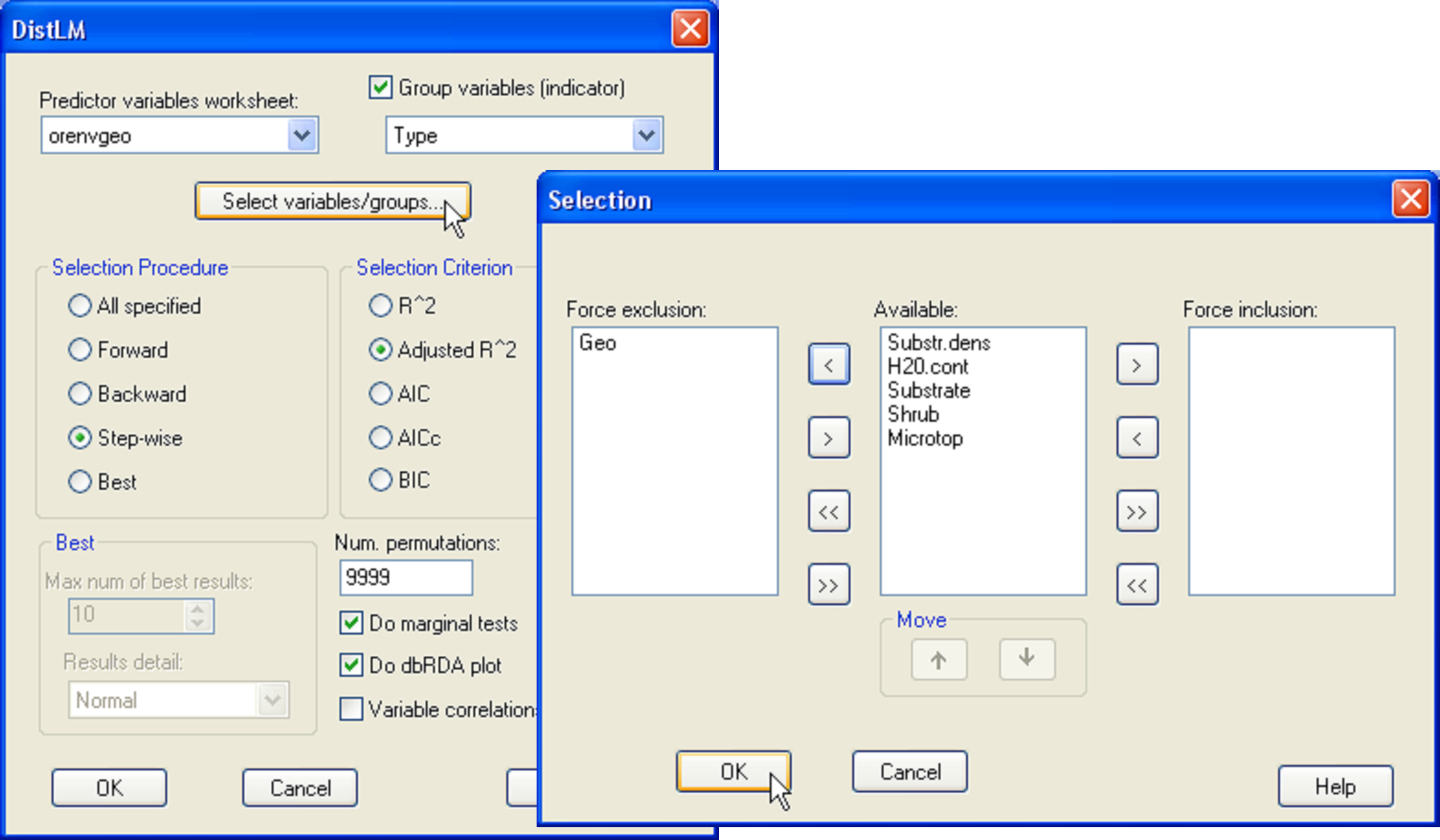
Fig. 4.24. DISTLM dialog for fitting the environmental variables (a mixture of quantitative and categorical variables) to the oribatid mite data, while excluding the geospatial variables.
Returning to the example, for simplicity we shall restrict our attention to the environmental variables only and omit the spatial variables from the analysis in what follows. The distributions of the categorical variables need not be considered using the usual diagnostic tools, as these only consist of 1’s and 0’s. A scatter plot using the draftsman plot tool in PRIMER for the two quantitative predictor variables alone (‘H2O.cont’ and ‘Substr.dens’) shows fairly even scatter and no indication that either of these variables requires any transformation prior to analysis. So, we are ready to proceed. First, calculate a Bray-Curtis resemblance matrix after square-root transforming the oribatid mite species abundance data. From this resemblance matrix, choose PERMANOVA+ > DISTLM > (Predictor variables worksheet: orenvgeo) & ($\checkmark$Group variables (indicator) Type) & (Selection Procedure •Step-wise) & (Selection Criterion •Adjusted R^2) & (Num. permutations: 9999) & ($\checkmark$Do marginal tests) & ($\checkmark$Do dbRDA plot). Before clicking the ‘OK’ button for the DISTLM dialog, force the exclusion of the spatial variables by clicking on the ‘Select variables/groups’ button and moving the group ‘Geo’ over into the ‘Force exclusion:’ column of the ‘Selection’ dialog (Fig. 4.24). The choice of adjusted R$^2$ as the selection criterion for this case is especially appropriate, because this criterion will take into account the fact that the sets of predictor variables have different numbers of variables in them, whereas the use of the raw R$^2$ criterion will not. If model selection were the ultimate aim, then one might alternatively choose to use AIC or BIC instead, which also would take into account the different numbers of variables in different sets. In our case, interest lies in determining how much of the variability is explained by each set of variables (thus the choice to examine marginal tests), and also what a sequential step-wise model fit of these sets of variables would produce.
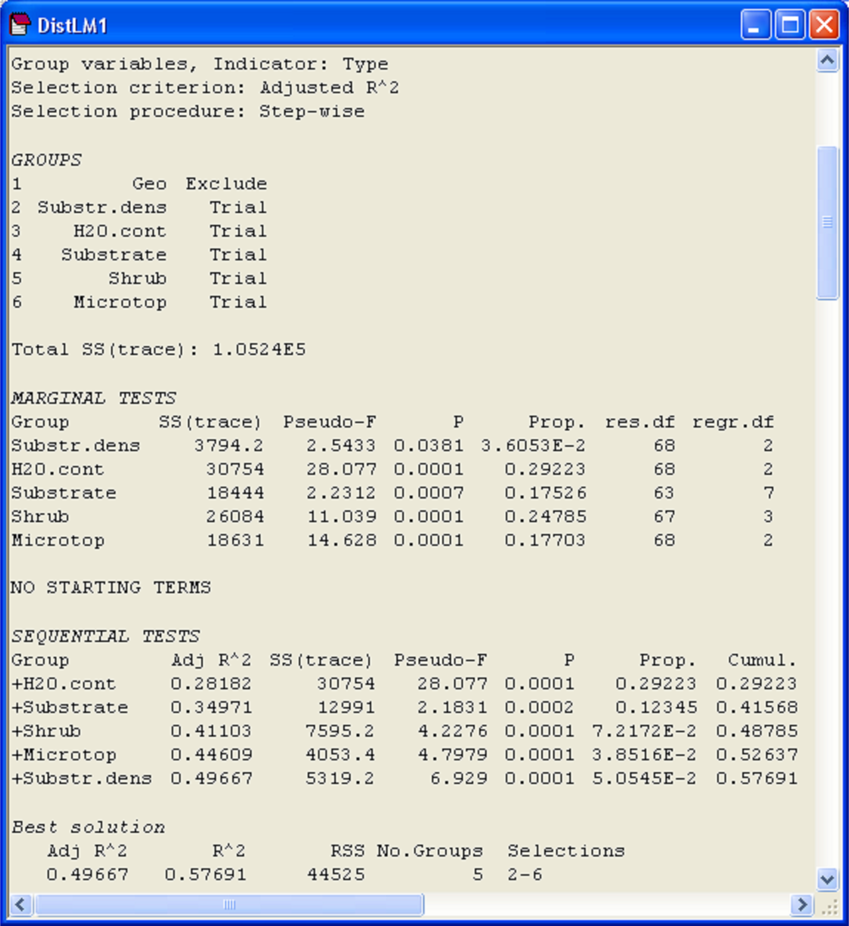
Fig. 4.25. Results of DISTLM for fitting the environmental variables (a mixture of quantitative and categorical variables) to the oribatid mite data, while excluding the geospatial variables.
Marginal tests (Fig. 4.25) show that each of the sets explains a significant proportion of the variation in the mite data, when considered alone (P < 0.05 in all cases). The single variable of water content (‘H2O.cont’) alone explains the greatest amount of variation in the oribatid mite species data cloud (based on Bray-Curtis), at 29.2%, while substrate density explains the least (only 3.6%). The set of variables that increased the value of adjusted R$^2$ the most after fitting ‘H2O.cont’ was ‘Substrate’, followed by ‘Shrub’, ‘Microtop’ and then ‘Substr.dens’. Although a step-wise procedure was used, at no stage were there any eliminations of sets from the model once they had been added and the conditional tests associated with each of the sequential additions were statistically significant (P < 0.001 in all cases). All of these predictor variables together explained 57.7% of the variation in the species data cloud and the adjusted R$^2$ for the full model was 0.497 (Fig. 4.25).
The full model can be visualised by examining the dbRDA ordination, requested as part of the output. The first two dbRDA axes captured nearly 80% of the variability in the fitted model, 45.7% of the total variation in the data cloud (Fig. 4.26). The vector overlay shows how the first dbRDA axis is particularly strongly related to water content, shrubs (none versus many) and microtopography (blanket versus hummock). When categorical variables are included in a DISTLM analysis, then the length of each categorical vector is a measure of the strength of the relationship between that category and the dbRDA axes. More particularly, if the separation of groups is clear in the plot, then we would expect the vectors for those categories to be relatively long. To help interpret ordination plots, it may be useful to provide the categorical variables also as factors; this will allow labels and symbols to be placed on the plot according to these different groupings. For example, by superimposing symbols corresponding to the three categories of ‘Shrubs’, a gradient from ‘none’ to ‘many’ (left to right) is apparent in the dbRDA diagram (Fig. 4.26). We leave it to the user to explore other categorical variables in this way, to examine unconstrained ordinations for the oribatid mite data and to consider analyses that might include the spatial variables as well.
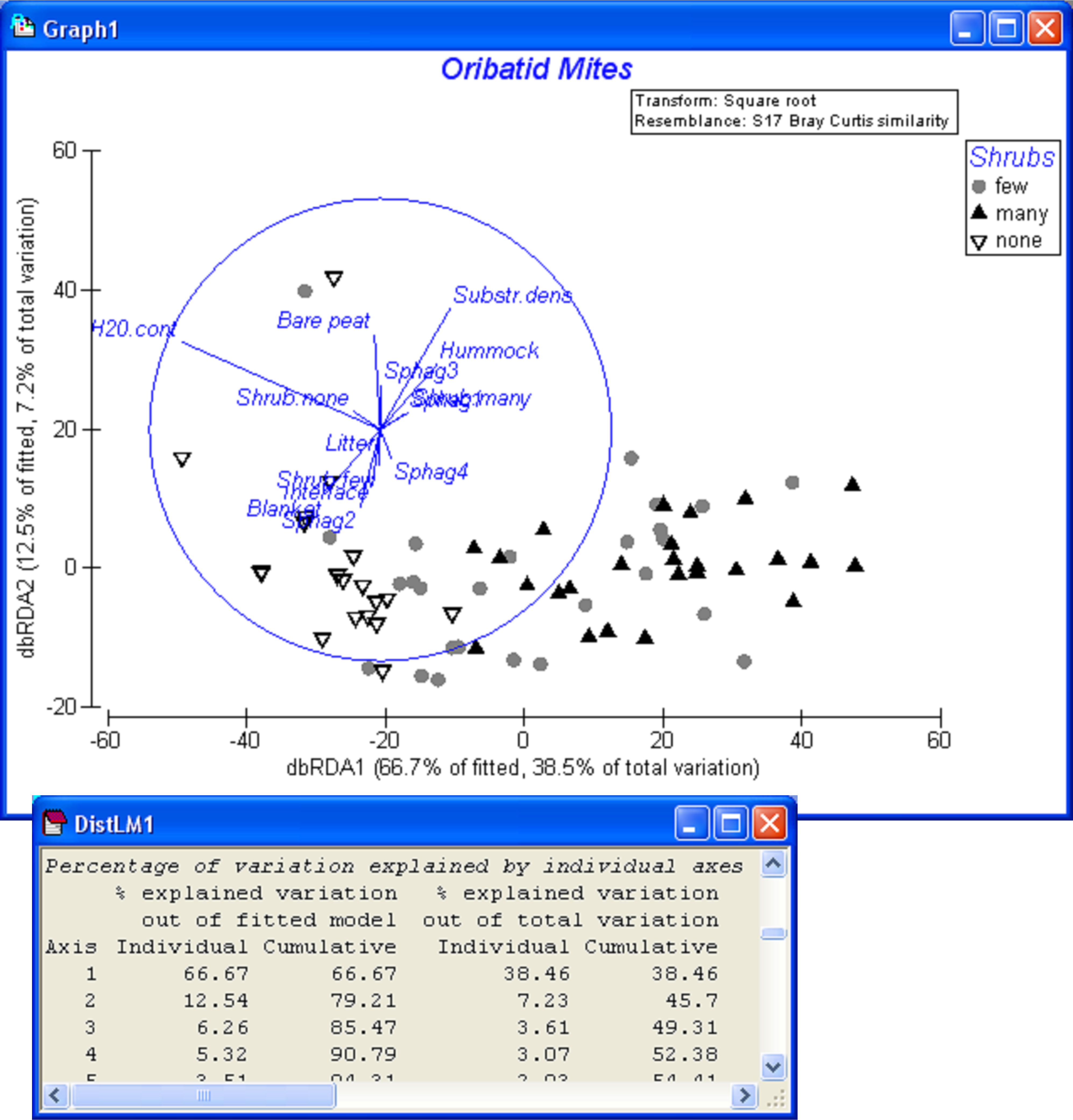
Fig. 4.26. dbRDA ordination for the fitted model of oribatid mite data (based on Bray-Curtis after square-root transformation of abundances) versus environmental variables.
94 This phenomenon is sometimes referred to as the “overparameterisation” of an ANOVA model.
95 The treatment of quantitative predictor variables as random (sometimes called “Model II” regression) does not exist within the current framework of either PERMANOVA or DISTLM and is a topic for further research. The CAP routine, however, is designed to examine the canonical correlations between two (sphericised) data clouds; it can be considered as one type of multivariate analogue to Model II regression. See chapter 5 for details.
4.16 DISTLM versus BEST/ BIOENV
On the face of it, the DISTLM routine might be thought of as playing a similar role to PRIMER’s BEST routine in the analysis of multivariate species data. More particularly, the BEST (BIOENV or BVSTEP) procedure in PRIMER is designed to find a combination of environmental variables which, together, result in resemblances among samples whose rank order best matches the rank order of the inter-sample resemblances arising from biological (species) data96. There are some important differences, however, between the BEST/BIOENV approach and models of a multivariate data cloud obtained using DISTLM.
First, DISTLM actually formally fits a linear model of the predictor (environmental) variables to the response (species) data cloud, in the space defined by the chosen resemblance measure. This means that the dissimilarities (or similarities) themselves are important here. They will define the shape and structure of the data cloud, so (as in PERMANOVA), the resemblance measure the user chooses is quite important. Indeed, although our ability to view the structure of this data cloud using unconstrained ordination (such as PCO) is necessarily imperfect, such an ordination should nevertheless be used to provide some information on whether there are any gross outliers, for example, which would make a linear modeling approach inappropriate. DISTLM does not assume anything specific about the shape of the data cloud, and any resemblance measure that is deemed appropriate for the nature of the data and hypotheses of interest can be used to construct it, but outliers or “high leverage” points97 in that space, if present, will tend to have a strong influence on the results.
The advantages of fitting a formal model using DISTLM are fairly clear. First, we achieve a direct quantitative partitioning of the multivariate variability that is explained by each of several environmental variables. Thus, we can determine how much of the variability is attributable to individual predictor variables (either acting alone or in pre-defined sets), and we can determine explicitly how much overlap there is in this explained variation. Of course, in order to do this, we have to be explicit about what we mean by “variation”, so that is where (and why) the choice of resemblance measure becomes so important.
Of course, DISTLM also has some clear limitations. First, despite the flexibility afforded by being able to choose any resemblance measure we wish as the basis of the analysis (so the models are usually not at all linear with respect to the original Y variables in the majority of cases), these models are strictly linear in the X variables. We can use polynomials of the X variables to get around this to some extent, but this is not the only potential issue. Another is that DISTLM’s reliance on the traditional partitioning approach means that we can run out of degrees of freedom if there are more predictor variables than there are samples. More particularly, in order to get sensible results, the largest possible full model is restricted to having q ≤ N – 1, at most. This is a simple consequence of it being possible to perfectly fit a linear model with (N – 1) parameters (variables) to N points (R$^2$ = 1.0). Although we can use criteria that are not strictly monotonic on R$^2$ with increases in predictor variables (such as adjusted R$^2$, AIC, AIC$_c$ or BIC), which will certainly help to find parsimonious models, all of the models fit by DISTLM partition the total variation using a linear function of the X’s and so will necessarily have this restriction of an upper bound on q.
In contrast, the BEST/BIOENV procedure arises out of the purely non-parametric approach inherent in the majority of the routines already available in PRIMER, such as non-metric MDS and ANOSIM. The differences between DISTLM and BIOENV are therefore directly analogous to many of the differences between PERMANOVA and ANOSIM already discussed in chapter 1. In essence, the BEST/BIOENV procedure does not attempt to model the data cloud at all, but rather tries to find the best possible rank-order match between the inter-point dissimilarities and the inter-point distances derived from sets of environmental variables. The criterion used for this matching is either a Spearman or a Kendall rank correlation, so it is only the rank orders of the resemblances that are being considered. There are several advantages to this approach. First, we can have as many variables as we want in either of the original matrices. The “matching” is being done on the basis of rank resemblances only, so there is simply no limit to how many original variables may be used to calculate either the species resemblances or environmental distance matrices. Second, the rank correlation (whether we use Spearman, weighted Spearman or Kendall) yields a criterion for the success of the match which (unlike R$^2$) is not monotonically related to the number of variables in the environmental data matrix at all. In fact, the inclusion of variables that do nothing to enhance the match will clearly cause a decrease in rank correlation. This criterion has intuitive appeal for identifying parsimonious sets of environmental variables that produce patterns among samples that are similar to the patterns produced among those same samples using the biotic data. Furthermore, the permutation test associated with the BEST/BIOENV routine includes the selection step with each permutation. This is really rather neat and allows the user validly to test the significance of the relationship between the two matrices given that some effort has gone into selecting environmental variables that will provide a good match.
The limitations of the BEST/BIOENV approach become apparent, however, when we realise that, once a purportedly “useful” set of environmental variables have been selected, we are not in a position to say how much of the variation inherent in the species resemblance matrix is “explained” by these variables, either individually or collectively. Such a variance is a function of the precise measurement scale of the resemblances, i.e. is a “metric” concept that cannot be captured by a non-(para)metric approach. The rank correlation between the two resemblance matrices does provide a valuable non-parametric index of how closely the collective set of environmental variables captures the multivariate pattern of the species variables (on a scale from $\rho \approx 0$ to 1), and this is an index with an absolute validity in comparisons across different transformations, resemblance measures, etc. (as with the similarly rank-based ANOSIM R statistic). However, it does not directly provide a quantitative measure of the relative importance of the individual environmental variables that have been selected; this can only be inferred by comparing the match ($\rho$) to the multivariate species cloud for different subsets of these environmental variables. Most tellingly, it cannot provide sequential (partial) tests, i.e. of the statistical significance of adding (or deleting) an explanatory variable from the current set. In other words, by going “non-parametric” (BEST/BIOENV), we relinquish our ability to explicitly measure and model multivariate variation. On the other hand, if we want to create such a model (DISTLM), then we must define what we mean by “multivariate variation” and decide how we are going to model it. This requires some decisions (e.g., which resemblance measure shall I use?) and some model assumptions (e.g., fitting linear combinations of predictor variables, and that the residual variability is additive and homogeneous across the different levels of the predictor variables). In short, we believe that DISTLM retains much of the flexibility of the non-parametric approach by allowing any (reasonable)98 resemblance measure to define what we mean by “multivariate variation”. However, in order to take the step towards formally modeling this variation, we are forced to let go of the fully non-parametric (and completely assumption-free) setting. Nevertheless, by using permutation procedures for the marginal and sequential tests, these additional assumptions can, however, entirely avoid being distributional.
96 See chapter 11 in Clarke & Warwick (2001) and chapter 11 in Clarke & Gorley (2006) for more details regarding these routines.
97 For a discussion of outliers and high leverage points in multiple regression, see for example Neter, Kutner, Nachtsheim et al. (1996) .
98 By “reasonable” we generally mean a measure that fulfills at least the first 3 of the 4 criteria of a metric distance measure (see the section Negative eigenvalues in chapter 3) and also one which is meaningful to the researcher for interpretation.