1.34 Types of sums of squares (Birds from Borneo)

When the design is unbalanced, there will be a number of different ways to do the partitioning, which will depend to some extent on our hypotheses and how we wish to treat the potential overlap among the terms. The different ways of doing the partitioning are called “Types” of sums of squares. More particularly, there are (at least) four types, known (perhaps unhelpfully) as Type I, II, III and IV. This terminology was initially coined by the developers of the SAS computer program (e.g., SAS Institute (1999) ), and is now in common usage. All of these types of SS produce identical results for balanced designs. Furthermore, Types II, III and IV will be identical for models with no interactions and Types III and IV will be identical if all cells are filled (i.e. if all cells have n ≥ 1). Searle (1987) provides an excellent text regarding models and hypotheses for unbalanced designs, including a comparison of the types of SS, which are briefly described below:

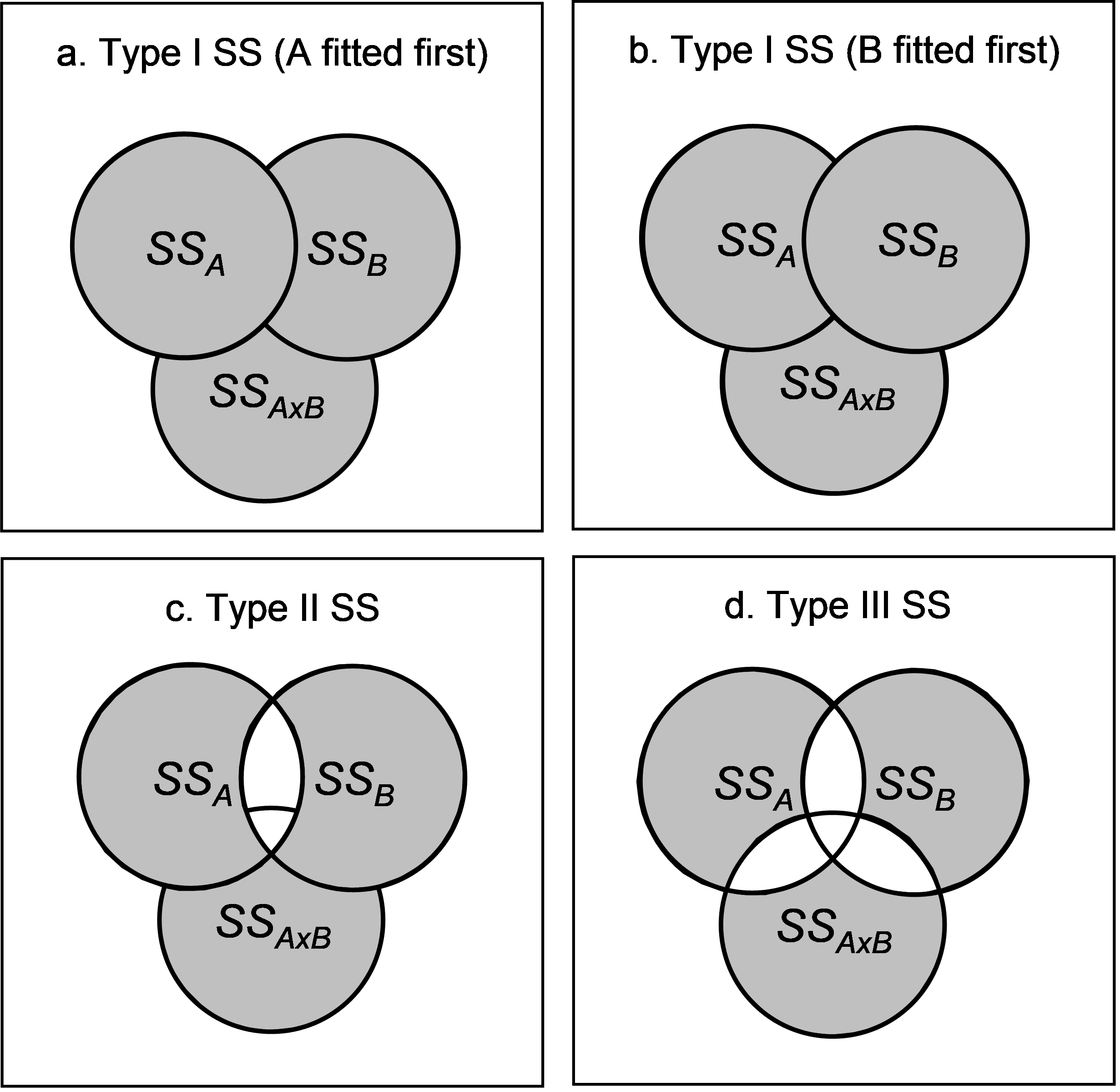
Fig. 1.41. Schematic Venn diagrams demonstrating the conceptual differences in Types of SS for a two-way crossed unbalanced design.

• Type I SS. This approach may be described as sequential. Here, each term is fitted after taking into account (i.e., conditioning upon or treating as covariates) all previous terms in the model. The order of the terms listed in the design file for the analysis therefore matters. For example, in the two-way crossed design, if the order of the terms listed in the analysis were A, B and A×B, then the SS would calculate the SS for A (ignoring other terms), the SS for B (given that A is already in the model) and then the SS for A×B (given that A and B are both already in the model). This is shown diagrammatically in Fig. 1.41a. You would get a different partitioning for this same design, however, if you chose to fit factor B first and then A given B (Fig. 1.41b). Another thing to note about Type I SS is that the sum of the individual SS will add up to the total SS. The sequential analysis offered by the Type I approach may be appropriate for fully nested hierarchical models, for which there exists a natural ordering of the terms. In other cases, Type I SS may be used to explore the amount of overlap in the explained variability among terms, by changing the order of the terms in the analysis and seeing how this affects the results.
   
• Type II SS. This approach might be described as a conditional analysis. The Type II SS for a given term is defined as the reduction in the residual SS due to adding the term after all other terms have been included in the model except any terms that contain the effect being tested. In other words, main effects are not conditioned upon interaction terms that involve them. In the two-way crossed design, this amounts to fitting A given B, B given A and A×B given both A and B (Fig. 1.41c). Note that, given the explicit definition, the order in which the individual terms are fitted will not matter here. However, the individual SS in the analysis will not necessarily add up to the total SS. There will potentially be some “bits missing” as a consequence of this partitioning. (In the two-way case, the “bit missing” is the overlap of factors A and B in their explained variation).
   
• Type III SS. This approach might be described as a fully partial analysis. Every term in the model is fitted only after taking into account all other terms in the full model. Thus, for our example, we can see this amounts to fitting A given both B and A×B, B given both A and A×B, and A×B given both A and B (Fig. 1.41c). Like for Type II SS, the nature of the definition here ensures that the order in which terms are fit will not matter. However, also like Type II SS, the sum of the individual SS will not add up to the total SS, and there will be more “bits missing” (ignored regions of overlap) for the Type III case. However, complete orthogonality (independence) of all of the hypotheses is ensured using this method.
   
• Type IV SS. This approach was developed by the SAS Institute (e.g., SAS Institute (1999) ) to deal with cases of a particular kind of imbalance known as “some cells empty”, in which data from some of the cells (combinations of treatments) are actually missing entirely (i.e. n = 0 for those cells). These situations can be contrasted with situations known as “all cells filled”, which may have either unequal or equal (balanced designs) replication per cell. According to Searle (1987) , Type IV SS are for testing hypotheses determined rather arbitrarily by the SAS GLM routine, which depends not only on which cells have data in them, but also on the order in which levels of the factors happen to have been listed. As such, Type IV SS is not generally recommended and is not discussed further here. The situation of “some cells empty” is quite adequately dealt with using Type III SS.

The PERMANOVA dialog box offers the user the option of using Type I, II or III SS. The default in PERMANOVA is to use Type III SS. This is primarily because most editors of journals (at least, most ecological journals) have now come to expect Type III SS to be used for unbalanced designs, simply because these will tend to be the most conservative of the three. However, there is no particular reason not to use the other types, especially if one of these is better suited to particular hypotheses of interest. For example, as already noted, a sequential analysis (Type I SS) would be quite sensible to use for an hierarchical nested design. Indeed, many statisticians would consider Type I SS to be the most sensible general approach, as no components of variation are left out (i.e. there are no “bits missing”). Type I SS also allows clarification of the relative sizes of overlapping regions, when terms are fitted in different orders. In most cases, provided the degree of imbalance in the design is modest (due, for example, to just a few missing observations here and there), the overall conclusions of the study will be little affected by this choice.
 

Fig. 1.42. Sample sizes per cell in the unbalanced two-way layout for the Borneo birds example.
 

A case in point is provided by an analysis of bird assemblages from Borneo, Indonesia in response to a two-way unbalanced design, as described by Cleary, Genner, Boyle et al. (2005) . A total of N = 37 sites were sampled within the Kayu Mas logging concession, close to Sangai, Central Kalimantan. The sites were cross-classified according to two factors: Logging (fixed with a = 3 levels: unlogged primary forest, forest logged in 1993/94 and forest logged in 1989/90) and Slope (fixed with b = 3 levels: lower, middle and upper). There were different numbers of sites (n) within each of the a × b = 3 × 3 = 9 cells in the design, as shown in Fig. 1.42. Within each site, spot-mapping (using calls and visual observations) was used to sample birds along each of two parallel 300 m linear transects, 50 m apart at each site. There were p = 177 bird species recorded in all and the data are located in the file born.pri, located in the ‘BorneoBirds’ folder of the ‘Examples add-on’ directory.
 

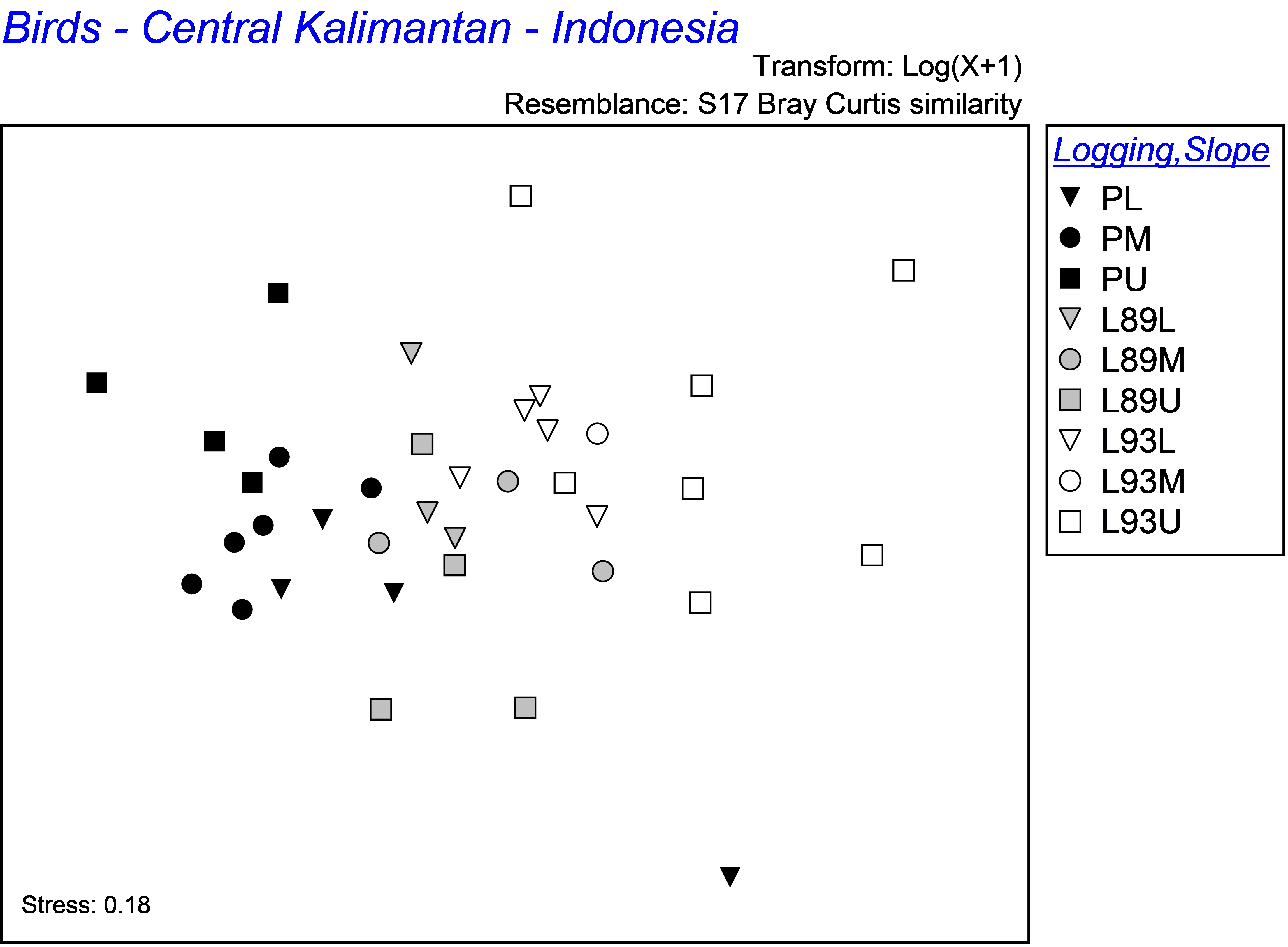
Fig. 1.43. MDS ordination of bird assemblages from Borneo in all combinations of logging (P = primary forest, L89 = logged in 1989/90, L93 = logged in 1993/94) and slope (L = lower, M = middle and U = upper).

An MDS plot of the bird communities, on the basis of log(x+1)-transformed data and Bray-Curtis similarities ( Cleary, Genner, Boyle et al. (2005) ) shows a clear effect of logging, and suggests some effects of slope as well, although these are less clear (Fig. 1.43). For illustration, four different analyses of the data were done using PERMANOVA (Fig. 1.44). First an analysis using Type I SS was done, fitting the factor of “Logging” first. Next, an analysis using Type I SS was done again, but this time fitting the factor of “Slope” first. Analyses were then done using each of Type II and Type III SS, in turn. Note that the SS for either factor using Type II SS corresponds to what is obtained if that factor is fitted second in a sequential (Type I) analysis. The Type III SS are different from all others, except for the interaction term, which in all cases was conditioned upon both of the main effects. Note also that the multipliers on individual components in each EMS differ for the different types of SS as well. This, in turn, means that the estimates of components of variation will also differ (Fig. 1.44).

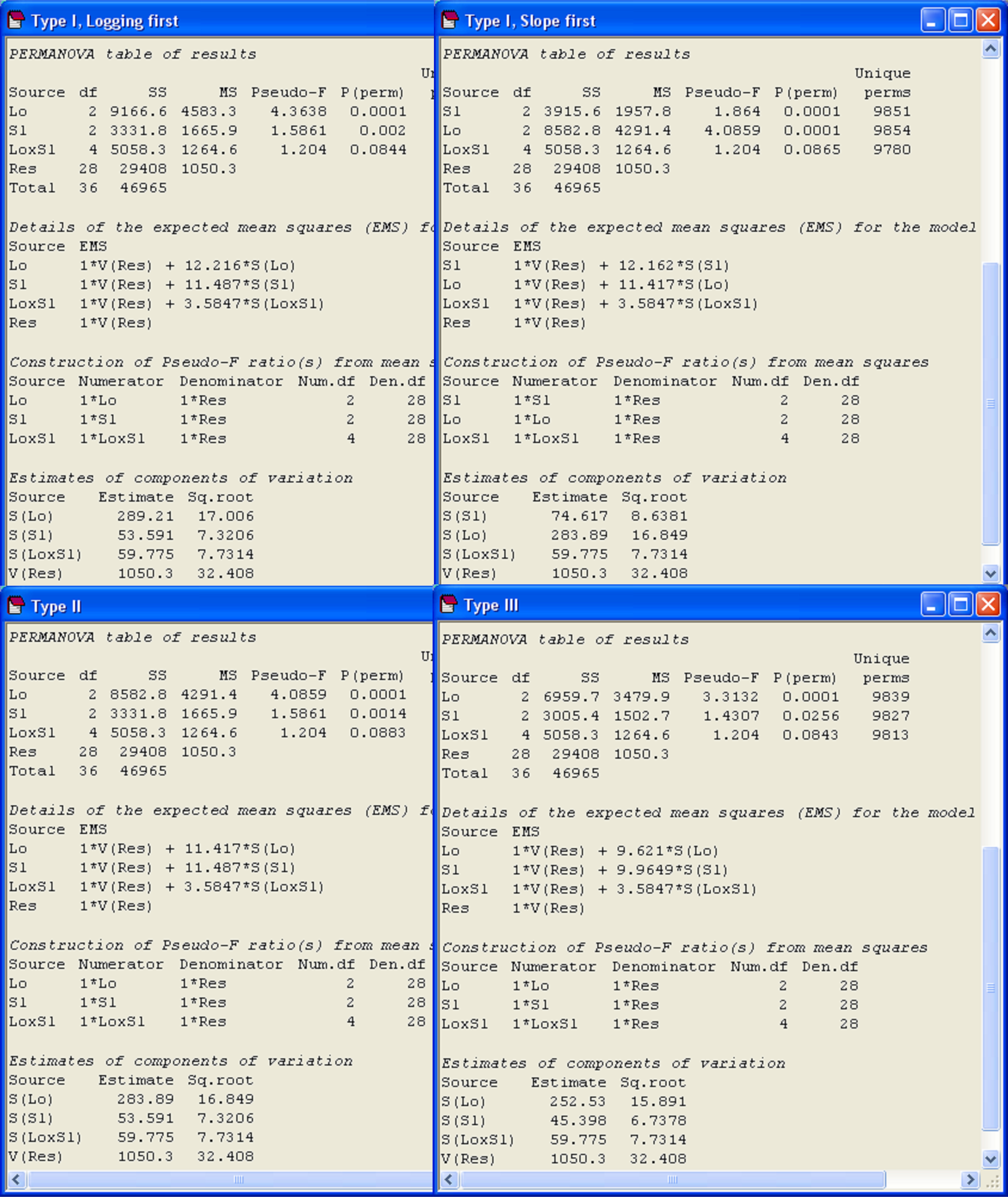
Fig. 1.44. PERMANOVA analyses of the two-way crossed unbalanced design for the example of Borneo birds using different Types of SS, as indicated.

In summary, the analysis of an unbalanced design using different Types of SS affects the values of (i) the SS themselves (and thus the values of MS and pseudo-F) for individual terms in the model; (ii) the EMS for each term and multipliers of individual components of variation; (iii) the estimates of the sizes of components of variation. Despite all of this, for the present example, the same general conclusions would be obtained, regardless of which Type of SS we had decided to use (Fig. 1.44). There are significant differences among bird assemblages in forests having different logging histories and the slope of the site also has a significant effect. These factors did not interact with one another and logging effects were much larger than slope effects (see Fig. 1.43 and also the estimated components of variation). The extent to which different types of SS will give comparable results will depend on just how unbalanced the design is – greater imbalances will generally lead to greater overlapping regions and thus potentially greater discrepancies. Perhaps the most important point is to recognise how different choices for the type of SS in unbalanced designs correspond conceptually to different underlying hypotheses (see Table 1.5, Fig. 1.41 and Searle (1987) ).

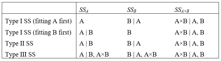
Table 1.5. Tests done using different types of SS in a two-way crossed unbalanced design (cf. Fig. 1.41). The vertical line is to be read as “given”, thus “A | B” should be read as “factor A given factor B”. A comma should be read as “and”.