1. Opening, editing and saving data (File, Edit)
- Getting the examples
- Primer file types
- Compatibility of files
- Opening the PRIMER 7 desktop
- Entering data directly
- Labelling samples & variables
- Deleting & inserting rows/cols
- Undo data sheet edits
- Moving & sorting rows/cols
- Cut, copying & pasting
- Saving data, renaming & deleting
- Undo in the workspace
- Saving, closing & opening a workspace
- Setting the initial directory
- Opening PRIMER files
- (Ekofisk oil-field fauna)
- Properties
- Opening Excel files
- (Ekofisk abiotic data)
- Wizard for input data
- Missing or zero values?
- (Tasmanian meiofauna)
- Opening several files at once
- Opening the same file twice
- Text-format input files
- Factors in 3-column text format files
- Dialog for input of text format files
- Size of data worksheets
- Merging worksheets
- Output data formats
- Editing labels
Getting the examples
The installation and subsequent run of Help>Get Examples V7 will have placed a number of sub-directories (BC zooplankton, Bermuda benthos, …, Wrasse diets) into the \Examples v7 directory, placed in a location which you have chosen. Throughout this manual it is assumed (for brevity) that the Examples v7 directory has been placed at the top level, i.e. the folder is C:\Examples v7. The various sub-directories contain the faunal matrices and, for some sets, the matching environmental data and taxonomy, for most of the case studies described in the Methods manual (CiMC: ‘Change in Marine Communities’, 3rd edition, 2014), and all the data sets in this manual. Check this by making sure you can find the directory \Examples v7\Fal benthic fauna, of the soft-sediment core samples of biota and matching environmental data for 27 sites from 5 creeks of the Fal estuary, subject to different levels of heavy metal contamination. That directory contains files such as Fal copepod counts.pri and Fal copepod taxonomy.agg, with similar files also for macro¬fauna and for the meiofaunal nematodes, all in internal binary PRIMER 7 format, and Fal environment.xls, an Excel sheet of variables $\times$ samples (though this could equally well be of samples $\times$ variables).
Primer file types
Whether the extensions *.pri, *.xls(x) etc display, or not, is a function of your Windows set-up; if you have suppressed them it is still easy to distinguish the different file types by their icon. There are PRIMER 7-specific icons and extensions for the following:
-
 (*.pri) sample data in rectangular format, and associated factors, description etc;
 -
 (*.sid) triangular matrices of similarity, dissimilarity, distance (generically, resemblances);
 -
 (*.agg) aggregation file, assigning species to genera to families etc;
 -
 (*.ppl) plot files, holding all the internal PRIMER information that structures the plot;
 -
 (*.pwk) workspace files of everything, so the PRIMER desktop can be reconstructed ‘as was’;
 - [
 (*.pdd) design files – these are only used in the separate PERMANOVA+ routines which are an add-on to the PRIMER software, see the separate PERMANOVA+ User Manual].
Compatibility of files
PRIMER 7 is fully forward-compatible from v6, and can input PRIMER 6, 5 and 4 data (*.pri and *.pm1), similarity (*.sid and *.sim) and aggregation (*.agg and *.pm1) files, and PRIMER 6 plot (*.ppl) and workspace (*.pwk) files, directly. But it is not, in general, backward-compatible so that PRIMER 6 cannot read workspaces, plot or data files saved in v7 format – there are many new plotting routines in PRIMER 7 that require additional internal data and graphic storage structures, workspaces from v7 in the earlier v6 format; little is lost with *.pri data files but, when such workspaces are re-opened in v6 (or v7), plot formats which are new to v7 will not be present, clearly. In addition, PRIMER 7 recognises several standard Windows extensions, e.g. input and output of *.xls(x) (Excel) and *.txt (text) data files or resemblance matrices; also *.csv, comma-separated text input. There are several options for *.txt text-format data input. Results windows can be saved in *.txt or *.rtf (rich-text) formats. PRIMER 7 can output plots to standard bitmap formats (*.bmp, *.jpg, *.png, *.tif, *.gif). An image in one of these formats can also be input to v7 (though with only minor use, as an image in an MDS bubble plot). Most usefully, plots can be output as vector-based enhanced metafiles (*.emf), and Copy and Paste operations from Graph windows in PRIMER to Microsoft Office routines (e.g. Powerpoint) are of this type, so plots can be ungrouped into Office drawing objects and further manipulated. PRIMER 7 also introduces some animation options, e.g. for spinning 3-d ordination plots, which can be output as movie files (*.mp4) or animated GIF (*.gif). All other file types (extensions) are not recognised.
Opening the PRIMER 7 desktop
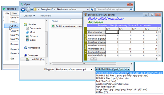
Start the program by (double)-clicking on the desktop or task bar PRIMER 7 icon ![]() , giving the window below. A second method is to double-click on a file with a recognised PRIMER extension, e.g. a worksheet file (.pri) or a workspace file (.pwk), and PRIMER 7 will automatically launch, with the selected file or workspace placed in the resulting desktop window. Note that opening more than one sheet by Windows Explorer>Open on a selection of filenames launches parallel PRIMER desktops, which is usually not the required outcome. To open multiple files simultaneously into the same workspace, first launch PRIMER then select several files in the File>Open dialog window.
, giving the window below. A second method is to double-click on a file with a recognised PRIMER extension, e.g. a worksheet file (.pri) or a workspace file (.pwk), and PRIMER 7 will automatically launch, with the selected file or workspace placed in the resulting desktop window. Note that opening more than one sheet by Windows Explorer>Open on a selection of filenames launches parallel PRIMER desktops, which is usually not the required outcome. To open multiple files simultaneously into the same workspace, first launch PRIMER then select several files in the File>Open dialog window.
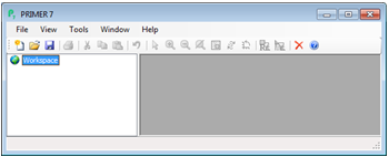
The PRIMER desktop is separated into two parts: to the left is the Explorer tree which will display icons for all the sheets, results windows, plots etc, and their interconnections. To the right, the actual worksheets, results and plot windows are displayed. The current workspace consists of all items in the Explorer tree (irrespective of which windows are displayed on the right hand side of the desktop), and all files needed for an analysis must first be opened into the current workspace.
Entering data directly
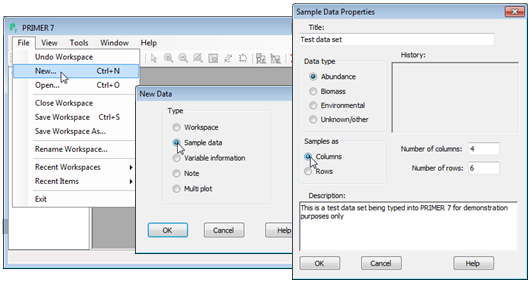
Most users will already have their data stored in rectangular form in some other software, e.g. as an Excel spreadsheet, which can be opened directly and straightforwardly (see later). However, data arrays can be typed directly into PRIMER, if necessary. Select File>New>(•Sample data) and, in the resulting Sample Data Properties dialog box, type in a title, specify a data type and which way round the matrix is to be, e.g. (Data type•Abundance) & (Samples as•Columns). You can also give a description of the data (optional), and you need to enter the number of columns and rows.
A worksheet of zeros is created into which you can type, by working down the columns, clicking on the first cell, typing in the number and pressing the Enter key. To edit an earlier entry, double click on the cell, amend it and again press Enter. To cancel an edit of a cell you have entered by mistake, press the Esc key. If you inadvertently click on a row or column label (the grey cells at the margins of the table) that row or column will be highlighted; remove the highlighting by clicking again on the label (highlighting is a simple on-off ‘toggle’).
Labelling samples & variables
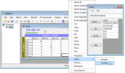
At this point only the default row (variables V1, V2, …) and column labels (samples S1, S2, …) have been defined, but a set of commonly used operations for worksheets can be found in the lower part of the Edit menu, including a Labels item. This menu can also be called up by right-clicking when the cursor is placed within the body of the worksheet (see below). The samples or variables can then be labelled: labels benefit from being succinctly descriptive; they must be spelt consistent¬ly from one sheet to another and unique within a sheet. This is because PRIMER 7 makes much use of label matching (e.g. abundance to biomass or species to environmental variables at the same set of sites, or the merging of species lists from different studies etc).
Deleting & inserting rows/cols
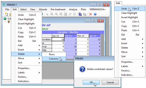
addition to attaching labels, the Edit menu allows a range of other edit functions on the data entries. For example, to delete whole columns (or rows), highlight them by clicking on their labels and then take a menu sequence such as Edit>Delete>Columns. A prompt is given for all such deletion operations to ask whether they were really intended. Note that the current cursor position – the cell in the sheet outlined in black – is ignored; deletion works only on highlighted rows or columns. In contrast, insertion ignores highlights and uses only the current cursor position, e.g. Edit>Insert>Row will add a new row immediately above the current position of the cursor and Edit>Insert>Column adds a new column to the left of the cursor. Logically therefore, if a new row or column is needed at the bottom or right of the whole data sheet, respectively, a different operation is required: this is Edit>Add>Row (or Column) and it will ignore the position of the cursor or any highlighting of rows or columns.
Undo data sheet edits
Occasionally, cell values are accidentally deleted or rows/columns added in unintended places but PRIMER 7 (unlike PRIMER 6) is able easily to back-track on such changes. There is a repeated Edit>Undo operation for all row and column manipulations on the Edit menu (between the Cut and Sort items). The Undo extends to any typing directly into cells of the data sheet or to copying and pasting rows/columns into it, whether from the same sheet or externally, from the clipboard.
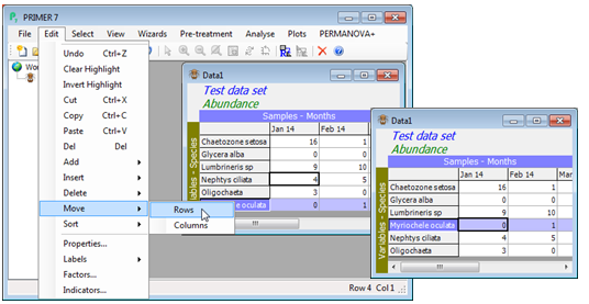
Moving & sorting rows/cols
Movement of rows or columns uses both highlighting and the cursor position. Rows (or columns) to be moved are highlighted, and the Edit>Move>Rows operation moves all high-lighted rows to immediately above the current cursor position when moving up, and below the cursor position when moving down (similarly with moving columns to the right or left – movement is always over the cursor). In the simple case illustrated below, the same outcome would have been achieved by Edit>Sort>Rows>(•By labels), since this is an increasing alphabetic sort of the row labels. Note that sorting can also be carried out according to some alphanumeric order, held in an indicator. The latter is the term that PRIMER uses for information associated with each variable – a catalogue numbering system here perhaps – see Section 2 on setting up factors and indicators).
Cut, copying & pasting
The Edit>Cut and Edit>Copy operations send part of a worksheet (or its factors/indicators) to the clipboard, where they are accessible by other Windows software or can be pasted back into another region of the active sheet (or factors). Cut and Copy operate much as in Excel etc, on highlighted regions of the worksheet, the difference here being that highlights must be whole sets of rows, or columns, or a combination of rows and columns, the highlighted data always being the darkest displayed cell colour (if nothing is highlighted the cell at the current cursor position is copied). Edit>Paste places the data from the clipboard onto a highlighted area of the same shape or, if there is nothing highlighted, onto a rectangle with its upper left corner at the current cursor position.
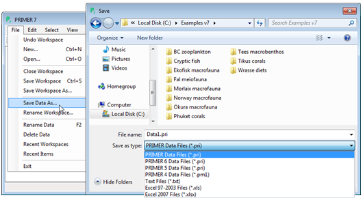
Saving data, renaming & deleting
The data sheet can now be saved (as can any item created in the workspace) from the File menu. File>Save Data As gives a standard type of Windows dialog box, shown below. This allows you to change to the desired directory, specify a meaningful name for the file (the default is Datan, where n just numbers each new data sheet in increasing order) and save it in PRIMER 7 format, with .pri extension, e.g. here in C:\Examples v7 and (File name: Test1) & (Save as type: PRIMER Data Files (*.pri)). This is the standard (binary) format for PRIMER 7 data matrices, which cannot be read by earlier PRIMER versions (including PRIMER 6) or by other software, but it is possible to choose to output in these earlier formats: PRIMER 6, 5 (Windows *.pri binary files) and 4 (the original DOS *.pm1 text file), plain text files (*.txt), and either the earlier Excel format (*.xls) with its restriction to 255 columns or the post-2007 *.xlsx format with no such constraints. On the same File menu there is an option to File>Rename the data sheet in the current workspace, or you can simply click once on the highlighted name box in the Explorer tree and overtype or edit the name. It is often a good idea to change the standard default names to something more meaningful in the context, so that you can find your way round the workspace more easily. Another option is File> Delete, which not only removes the specific data sheet from the workspace (though does not delete it in the original directory of course!) but also removes all the structure which leads immediately from that sheet (data sheets, results or graphs on the same branch of the Explorer tree, Section 7).
Undo in the workspace
Another new feature to PRIMER 7 is the option Undo Workspace which back-tracks for the work¬space operations of renaming or deleting any sheet (or other window), or renaming the workspace.
Saving, closing & opening a workspace
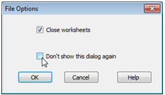
 Typically, a single workspace would encompass one or more inter-connected data sets which are analysed at the conclusion of a specific phase of a study (unrelated data sets and analyses are best handled in separately created workspaces). Thus, rather than saving individual data or results files, more useful is the ability in PRIMER to save entire workspaces. This can be accomplished initially with File>Save Workspace As, which gives a Save dialog box similar to the above, but producing *.pwk file types, which are internal binary formats not accessible by any other software. By default this saves a PRIMER 7 workspace format, capturing all the data, results and graphical structures, and their links, as represented in the current state of the workspace. (Subsequent workspace saves with the same name, overwriting the existing copy, are carried out with File>Save Workspace). An alternative is to save the workspace in PRIMER 6 format (also with a .pwk extension), within which many of the new features in v7 cannot be represented and are therefore omitted, though the file can then, of course, be opened by users working only with the earlier PRIMER 6. In general, it is only the new graphic formats which are lost, with the basic tree structure of the analyses and the results windows being retained. More detail about managing workspaces, and exploring the links between component items, is given in section 7 but, for now, note that other functions frequently used are File>Close Workspace (or File>New>Workspace), which leaves a new, clear workspace ready for opening of new files (and will prompt for a Save Workspace operation unless one has just been carried out), and opening an already saved workspace (either of PRIMER 6 or 7 format) with File>Open. For the latter, after the usual dialog to select a *.pwk workspace file, taking the tick box option (✓Close worksheets), see below, suppresses the roll-out of the branches of the Explorer tree, so that just the top-level worksheets in the workspace are shown, prefixed by
 ![]() , and sheets are not displayed on the PRIMER desktop. (Clicking on the plus signs, successively, will unravel the full tree structure). This is a potentially useful new feature in v7 which speeds up opening of a large workspace, which was saved with very many sheets open on the desktop. It is not the ‘factory default’ but once selected this becomes the default option for opening the next workspace, even for a new run of PRIMER. For a consistently preferred option here, this dialog box can be eliminated.
, and sheets are not displayed on the PRIMER desktop. (Clicking on the plus signs, successively, will unravel the full tree structure). This is a potentially useful new feature in v7 which speeds up opening of a large workspace, which was saved with very many sheets open on the desktop. It is not the ‘factory default’ but once selected this becomes the default option for opening the next workspace, even for a new run of PRIMER. For a consistently preferred option here, this dialog box can be eliminated.
The test data matrix saved above is too small to do anything useful with, typical species by samples matrices often having hundreds of species or samples. So, take File>Close Workspace and we shall now work with a real 174 species by 39 samples array (Ekofisk macrofauna counts.pri), of soft-sediment macro¬faunal abundances, in PRIMER 7 format, and a matching 39 samples by 9 environmental variables matrix (Ekofisk environment.xls), in Excel format, both files being in the directory C:\Examples v7\Ekofisk macrofauna.
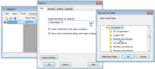
Setting the initial directory
It may sometimes be convenient to set the initial (default) directory to which PRIMER 7 opens every time it is run. Here this would use Tools>Options and supply (or browse for) the directory C:\Examples v7\Ekofisk macrofauna, see below. (Note that this run of PRIMER has to be shut down before the default change is implemented for future runs of PRIMER). For this tutorial, the default might logically be set to C:\Examples v7. Often, however, it is more convenient to leave this box blank and the program then always defaults to the previously used directory. (Incidentally, the Tools>Options dialog also gives the option to reverse the decision made in the illustration above, to eliminate the (✓Close worksheets) dialog box on opening a saved workspace.)
Opening PRIMER files
File>Open>(File name: Ekofisk macrofauna counts.pri)>Open will read in the existing Ekofisk species-by-samples array. The default file types are any of the PRIMER 7 formats, though earlier formats (Windows PRIMER v6 & v5, DOS v4), text and Excel files (commonly used for initial data input) are available. These are listed in detail on the first page of this section (Section 1).
(Ekofisk oil-field fauna)
The abundance file Ekofisk macrofauna counts.pri is displayed within the PRIMER desktop. It shows the typical sparseness of species matrices, with many zeros and some large counts, each sample being the total of three Day grab samples at each site and the sites, S30, S36, S37, S31, … being ordered left to right in increasing distance from the centre of oil drilling activity – the design is roughly that of five radial transects from the centre of the oilfield out to distances of 8 km, at geometrically increased spacing. See Chapters 10 and 14 of the CiMC manual for a diagram of the sample sites and other details of this study (original paper: Gray JS, Clarke KR, Warwick RM, Hobbs G 1990, Mar Ecol Prog Ser 66: 285-299).
The data matrix, and any window in the PRIMER desktop, can be resized by dragging a corner of the window, as for the desktop itself, in normal Windows action. Note that by clicking on any cell in the matrix, its row and column numbers are indicated at the bottom right of the desktop.
Properties
Edit>Properties produces the Sample Data Properties dialog box, seen earlier, where information about the data can be checked and amended, e.g. Title, Data type, Description, numbers of rows and columns and that the Columns are the Samples in this case. The History box will accumulate information on Pre-treatment operations such as standardisation, transformation, species weighting etc (and for resemblance matrices will specify the coefficient used). Properties is also one of the items that can be selected by right-clicking over the data sheet.

Opening Excel files
Usually, rectangular data matrices of variables by samples, or samples by variables, will initially have been entered into Excel. For entry to PRIMER, these should have different data arrays (e.g. abundance, biomass, environmental variables etc) in different sheets – though they can be in the same Excel file – and will need to be read in one sheet at a time. The data format is simple but specific and must be adhered to. For the above Ekofisk counts, an Excel file would have been:
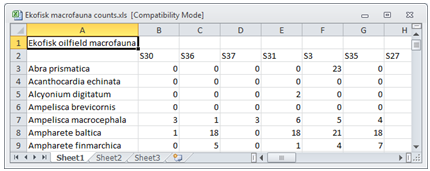
If referring to the same set of sample locations/times/treatments/replicates, different biotic and abiotic arrays should have the same (unique) sample labels over the different sheets; the samples can then be matched. The label would helpfully be a combination of the particular location/time/ treatment/replicate alphanumeric codes, though it could be a simple integer code (1, 2, 3, …). Either way, the place to identify the different factors (location, time etc – see Section 2) is not as multiple heading rows at the top of the matrix (only one row of sample labels is allowed) but at the bottom of the array, separated from the data by a blank row. The data array can be entered as the transpose of that shown above (samples as rows rather than columns) but the same principle applies – any factors are placed to the right of the data separated by a blank column (in practice, a blank column label is sufficient to make PRIMER believe that the data has finished and the factors started, so you must avoid using a blank sample label). An example of the environmental data for the Ekofisk study, in this transposed format, is now used to step through the input options.
(Ekofisk abiotic data)
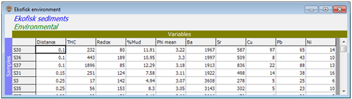
For the 39 sites around the Ekofisk oil-field, environmental data is available on concentrations of total hydrocarbons and metals such as Barium, Strontium, Copper in the sediments, and measures of physical sediment properties, such as % mud; also the distance from the oilfield centre is another variable in this array. These are in the Excel file Ekofisk environmental.xls:
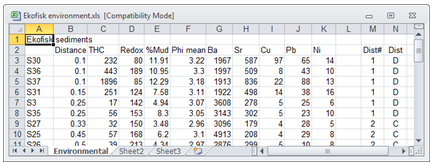
Note that there is only one sheet defined in this case (‘Environmental’), it is in the form samples variables with the same (unique) labels for the sites as in the assemblage data, which can be of any length and consist of a mix of numbers, letters and spaces (as can the title be, if present), but data entries must always be strictly numeric (e.g. ‘<’ signs are not permitted).
Wizard for input data
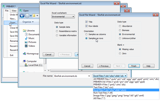
File>Open gives the same Open dialog box as previously but, importantly, the drop down menu on the bottom right of this dialog should now be used to select files of type: Excel Files (*.xls, *.xlsx, ..), otherwise the Excel file will not be visible in the file listing. Click on a filename and the Open button generates a ‘wizard’ which guides the user through the choices that must be specified. On the first dialog box, specify which Excel worksheet to use from the file, selected by name, and then what Data type: •Sample data (a rectangular array of samples $\times$ variables or variables $\times$ samples); •Resemblance matrix (a triangular matrix of pairwise similarities/dissimilarities/distances/ranks/ correlations and even pairwise ANOSIM R statistics – PRIMER will itself generate a wide range of these from sample data sheets but it might, for example, be required to input a specialised measure computed by other software into the PRIMER routines); •Variable information (this is a slightly broader category in PRIMER 7 which is still, however, mainly used to hold taxon information on each species, referred to previously as aggregation files, in which species are linked to their taxon¬omic hierarchy of genus, family, order, etc).
On the second dialog box, make sure the Title box is checked (the default option) if there is a separate title line in the top left cell (A1) of the Excel file. Failing to uncheck this box when there is no additional title line is likely to be the commonest source of problems when reading an Excel sheet into PRIMER, the first row of the data matrix then being mistaken for the column labels (also, failing to check the box when there is a title will result in blank input sheet). Similarly there is a check box for the presence of row labels, e.g. species names (which is the default since they are almost always present). Other choices in this dialog specify whether the Samples are to be taken as columns or rows, and whether the data is of Abundance, Biomass, Environmental or Unknown/ Other type. This Data type designation is not crucial, but it does allow PRIMER 7 to select natural defaults for analysis choices, e.g. of resemblance coefficient, dependent on specified data type.
To input the above Ekofisk environmental matrix from the C:\Examples v7\Ekofisk macrofauna directory, take File>Open>(File name: Ekofisk environmental.xls)>Open>(Excel work¬sheet: Environmental) & (Data type•Sample data)>Next>(✓Title) & (✓Row labels) & (Orientation •Samples as rows) & (Data type•Environmental) & (Blank=•Missing value)>Finish, as shown:
Missing or zero values?
The final option is whether a blank cell in the Excel sheet should be interpreted as a Missing value or a Zero. Typically, it will be Zero for species variables and Missing for environmental or other data. The distinction is important for subsequent analysis: most species-by-samples matrices have large numbers of species that are not present in many samples – they are indicated by zeros, and this information is properly catered for by an appropriate choice of similarity coefficient. If an environmental variable is not detected at a sample site then that should also be recorded as a zero, or as the lower detection limit (or perhaps half that limit). If a specific variable is not measured at a site, through random loss of a sample, then that is properly a Missing value. Inputting a blank cell from Excel, with the (Blank=•Missing value) option, or editing it to a blank after it has been read into PRIMER, will display a Missing! entry.
There are then three possible approaches. For environ¬mental type data which might be transform¬able to approximate multivariate normality, and for which there are relatively few missing cells, a good option may be to attempt statistical estimation of the (randomly) missing values using the Tools>Missing routine. This uses the EM routine to give maximum likelihood estimates of the missing cells by exploiting the correlations among variables (see Section 12), thus completing the matrix. However, in many cases these normality assumptions are not viable, or there are simply too many parameters to estimate. Thus, secondly (and new to v7), PRIMER now automatically takes the simpler approach of calculating resemblance measures after removing, separately for each pair of samples, all variables which have a missing value for either sample. All resemblance measures are then auto¬matically adjusted for the crude bias which results from such pairwise eliminated data input to totalled measures, such as Euclidean and Manhattan distance (without this adjustment some pairs of samples would be given greater distance simply because they are summed over more variables), see Section 5. Of course, a third possibility is simply to select a subset of samples and variables for which there are no missing values, e.g. by Select>Variables>(•No missing values).
It is important to appreciate that random loss of a whole sample (for all variables), e.g. loss of a replicate community sample from a balanced sampling design, is not thought of as producing missing values. If all species (or variables) are lost for that sample, it is simply omitted, and the design becomes a slightly unbalanced one, which is perfectly well catered for in most of the PRIMER (or PERMANOVA+) routines, e.g. in the ANOSIM or PERMANOVA hypothesis tests.
Save the workspace in the C:\Examples v7\Ekofisk directory with File>Save Workspace As>(File name: Ekofisk ws.pwk), for later use, and File>Close Workspace to clear the workspace. Further files will now be opened from C:\Examples v7\Tasmania meiofauna, to demonstrate text file input.
(Tasmanian meiofauna)
This study concerns meiofaunal abundances from a two-way layout of samples on a sand-flat in Eaglehawk Bay, Tasmania, see Chapters 6, 7 and 12 of the CiMC manual. Separate data arrays are available of nematode and copepod communities associated with disturbed and undisturbed patches of sediment at four locations across the sandflat, the disturbance being caused by natural burrowing activity of soldier crabs (original paper: Warwick RM, Clarke KR, Gee JM 1990, J Exp Mar Biol Ecol 135: 19-33). The two disturbance conditions (D and U) are referred to as the treatments (though this is an observational study not a manipulative experiment) and the four locations as blocks (B1 to B4). For each treatment/block combination there are two replicates. Each replicate is a sediment core for which both nematodes (39 taxa) and copepods (17 taxa) are counted.
Opening several files at once
The directory C:\Examples v7\Tasmania meiofauna contains the PRIMER 7 files of separate nematode and copepod data, Tasmania nematodes.pri and Tasmania copepods.pri. Both can be opened in one step by taking File>Open and clicking on these file names, with the Shift or Ctrl key held down. (This operates in the usual Windows way, with Shift-click highlight¬ing all files between the two items selected, and Ctrl-click highlighting individual, non-consecutive files in the list.) Both (in general, all) selected names appear in the File name box and are opened with a single press of the Open button.
Opening the same file twice
PRIMER 7 will allow the same file to be opened into the workspace more than once, since the response to the Open menu item is to create a copy of the file for entry to PRIMER at that time, and there is no physical link maintained from the workspace to the original file. Thus amendment of that external file cannot alter data entries in the workspace, and vice-versa (unless, of course, Save Data As is used to overwrite that file with one of the same name), so a second copy of the original file can be opened without difficulty. PRIMER 7 does, however, demand unique naming of all workspace items, so any second (and subsequent) attempts to open the same file will add a version number, e.g. Tasmania copepods(2). Similarly, default names for new windows generated automatically by an analysis sequence: Data1, Data2, …, Resem1, Resem2, …, Graph1, Graph2, … are unique, and if changed to more identifiable names, these too should be unique. Thus an attempt to give the name Tasmania nematodes to a similarity matrix as well as the data sheet will result in the name Tasmania nematodes(2) being assigned.
Text-format input files
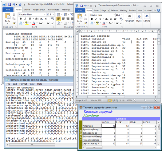
The Tasmania meiofauna directory also contains three different text format versions of the copepod samples, Tasmania copepods tab-sep.txt, Tasmania copepods comma-sep.csv and Tasmania copepods 3-column.txt, in addition to a fourth text version of the same data, Tasmania copepods v4.pm1, which is in the original DOS PRIMER v4 format. The first two are rectangular variables $\times$ samples (but could be samples $\times$ variables) arrays, and differing really only in what is used as a separator (delimiter) between the data entries: *.csv files are comma-separated and *.txt are typically tab-separated (e.g. outputting to *.txt format gives tab delimiters). However, input from *.txt format is more general: it can also cater for comma-separated or space-separated entries or the use of any other specified delimiter. In all cases, rows are separated by (hard) carriage returns but for columns there is no limit on the length of each line, and these will typically be wrapped (with soft carriage returns) when displayed with a text editor or word processor, as seen below. The third file, Tasmania copepods 3-column.txt, is an example of 3-column format, in which each line of the text file has only three columns of data separated by tabs (other delimiters, such as commas, are also allowed). The format must again be followed exactly: as the second line of header information shows, Column 1 is the sample label, column 2 the variable label, and column 3 the numeric data entry. The advantage of this format is that only non-zero entries need be listed – when PRIMER converts this to rectangular format the blank cells will be automatically filled with zeros (and again without fixed size limits). Importantly, this ‘flat-form’ structure is the record format which many relational databases use to hold observed occurrences or counts of a specific species at a specified location (set the third column to 1 throughout, if these are records only of presence), and the same record format is often also used for abiotic or other measurement variables. All such databases (e.g. Access) will be able to output comma/tab separated text format files of the type shown below right.
Factors in 3-column text format files
Associated with each record are often one or more factors which define the conditions under which that sample was taken (sites, times etc). These could be copied and pasted from a sample table held in the relational database to a factors sheet set up for that data in PRIMER – see section 2 for how to set up factors within PRIMER – but this categorical information on the data structure is typically output from the relational database as part of each record. If there is no access to the original data¬base table of factors, such a record format can be used by PRIMER 7 to populate its factor table. This is why the above 3-column example does not contain just three columns, in this case! There is a fourth blank column (i.e. an extra tab) and then two (alphanumeric) factor level columns – though there could be many more – which here define the block and disturbance status for each record. Of course each combination of the two factor levels is repeated as many times as there are numbers of species observed in that sample, and if these entries are not identical an error message will result. Then (if needed) follows another blank column (extra tab) and any ‘factor levels’ defined on the variables (termed indicators, see Section 2); here this indicates which species have been identified.
Dialog for input of text format files
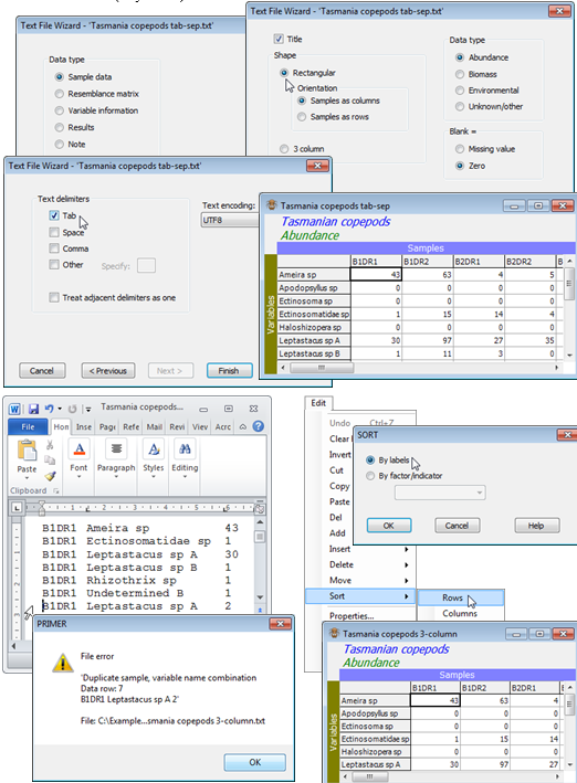
Read in the first of the above text files: File>Open>(Files of type: Text Files (*.txt, *.csv)) & (File name: Tasmania copepods tab-sep.txt), using the Text File Wizard dialogs shown below. Repeat for Tasmania copepods comma-sep.csv, the only difference being the switch to (Text delimiters ✓Comma) in the third dialog box. For Tasmania copepods 3-column.txt, the below shows the error message obtained having inserted at line 7 a mistaken repeat of the same combination, ‘B1D1R1 Leptastacus sp A 2’. When the error is corrected, the Wizard dialog proceeds exactly as for the other two cases, except that the option (Shape•3 column) is selected in the second box. Note that the 3-column file enters PRIMER with a different species order (the order in which variable names are encountered in the file); it will coincide if rows are re-ordered alphabetically with Edit>Sort>Rows>(•By labels).
Size of data worksheets
There are no fixed size limits for arrays within PRIMER 7, simply an overall limit determined by the amount of available real memory on the computer. There will, of course, be significant time constraints for some of the more compute-intensive routines, and there is a limit to how many samples it is sensible to try and view at the same time, in ordination plots for example, but it is a viable strategy to place all related data into a single workspace, and data of the same type (e.g. counts for a specific faunal assemblage in a complete set of samples) into a single worksheet. Defining a structure of factors on the samples (see Section 2) will allow the selection of subsets from that worksheet, or averaging over replicates (or factor levels), needed for a specific analysis. Continually improving computational power makes it possible at least to hold and manipulate arrays with thousands of species (typically OTU’s in microbial applications) and thousands of samples, even if successful analyses will often involve targeted selections or averages of samples. Whether matrices are input as samples (rows) $\times$ variables (columns) or variables $\times$ samples is not of relevance: PRIMER simply needs to be told whether the samples are the rows or the columns. Note that transposing a worksheet within PRIMER is possible (by Tools>Transpose), but will not correct a mistaken attribution on entry – if the rows have been incorrectly called ‘samples’ during the Open dialog then, after transposing the worksheet, the columns will still incorrectly be called ‘samples’. Instead, the mistake is corrected by Edit>Properties and taking Samples as•Columns.
Merging worksheets
For data collection reasons, it may still be the case that data from essentially the same array are sourced from several different file, e.g. abundance of comparable species lists over a set of sites but with data from different years held in different Excel sheets. If those sites, or some of them, need to be analysed over the years then the best strategy is often to read all the different files into PRIMER and then Tools>Merge them to a common worksheet. Before entry, the sample labels should be unique, e.g. identify the year as well as the site and the replicate number etc, and species names (or numbers) be consistently spelt. Then runs of Merge will stitch the sheets together, a pair at a time, expanding the species lists accordingly to take account of the fact that different years may have species lists of slightly different composition, length or order, and zeros will be added in relevant cells (or Missing! if this is selected as more appropriate, e.g. as it would be for environmental data). Not all data for the same set of sample labels should necessarily go into a single worksheet, e.g. species abundances and environmental variables for the same set of sites/times are usually best kept in separate arrays because sample resemblance matrices (Section 5) will often need to use different coefficients. Whether environmental information is best held as a separate data array or as a factor sheet associated with a species array depends on the data type and context: factors are categorical (whether unordered or numerically ordered) whereas data arrays are numerical. Some variables may appear in both ways, e.g. water depth in an abiotic matrix and as a factor (shallow, mid, deep).
Output data formats
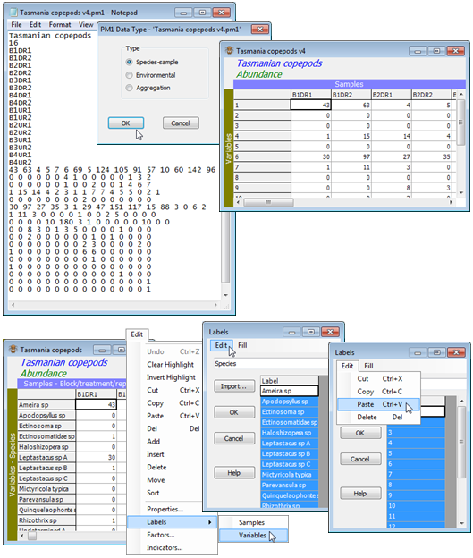
Output format options, with File>Save Data As, are generally the reverse of input choices. The default is a PRIMER 7 (binary) file but data sheets (or resemblance matrices) can also be saved in earlier PRIMER 5 and 6 binary formats, and to Excel in current *.xlsx format or the older *.xls (with its restriction to < 255 columns). Text files can also be output in either rectangular or 3-column format, the separators then always being Tabs. The very early DOS PRIMER 4 text format can also be output (or input) but much of the associated information (e.g. species names, factors) is lost, and this format is likely only to be of interest at this stage in restoration of old archives. An example of the PRIMER 4 format can be seen in the file Tasmania copepods v4.pm1 below, which contains the same counts as Tasmania copepods.pri though cannot hold species names or factors in the same file. (Note that line 2 defines the number of samples, followed by the sample labels and then species counts separated by any combination of single or multiple spaces or tabs).
PRIMER 5 files did not have a defined data type (so are all read in by PRIMER 7 as Data type• Unknown/other). They also had no History box (defining standardisations, transformations etc which may have been applied to obtain the current sheet). It follows that outputting PRIMER 7 files in PRIMER 5 format will lose the information on Data type and History. As noted at the start of the section, in contrast, differences between PRIMER 6 and 7 data formats are rather minimal (though workspace files are very different). However, PRIMER 7 is not backwards-compatible in general, so that PRIMER 6 cannot open files created in PRIMER 7 unless they have been explicitly saved to the earlier format. Naturally, PRIMER 7 is forwards-compatible and will automatically open any earlier data or v6 workspace files.
Editing labels
Take File>Open>(Filename: Tasmania copepods v4.pm1)>Type•Species-sample to input this (archival) v4 format file, and note that the missing species labels could be copied and pasted from elsewhere (if they were available in the same order) – perhaps an external file or, as demonstrated below, from another worksheet within the workspace (Tasmania copepods.pri). All amendments to labels are implemented through Edit>Labels>Variables (or Samples), then clicking on the label header will highlight the full set of labels for copying out – or pasting into – their contents.
Save the current workspace in the C:\Examples v7\Tasmania meiofauna directory, with File>Save Workspace As>(File name: Tasmania ws.pwk), for use in the next and later sections.