11. General data manipulation (Tools, further Pre-treatment)
- Tools vs. Edit menu
- Average and Sum on data matrices; Average on resemblance matrices
- Aggregation
- Check on aggregation files
- Tree menu; Check on datasheets & resemblances; Undefined resemblances
- Duplicate; Merge (/join) operations
- (Tasmanian meiofauna)
- Combined cells in Merge
- Avoiding strict label matching
- Merging non-uniform species lists; (Phuket coral reefs); (Clyde dump-ground study)
- Missing data estimation
- EM algorithm assumptions
- Missing data estimation (Clyde study)
- Ranked variables
- Ranked resemblances
- Transposing the datasheet
- Transform (individual) advanced
- Expressions combining variables
- Expressions combining worksheets
- Average body mass matrix (B/A)
- Transform on resemblances; Combining resemblances
- Tools menu - other items; Tools Options menu
Tools vs. Edit menu
Both the Edit (see Section 1) and Tools main menus carry out ‘housekeeping’ manipulations on a dataset (or a resemblance or variable information sheet, such as an aggregation file). The operations are usually rather straightforward, and with an obvious outcome, as opposed to the Analyse menu which contains the primary statistical routines. The main difference between Edit and Tools is that items on the main body of the Tools menu create a results window, and in most cases also produce a derived sheet of the same type, e.g. a new data sheet from a data sheet. (There are two miscellaneous items at the bottom of the Tools menu, Stop Tasks and Options, which do not fit into these rules, but are there because this is the conventional place for them in Windows applications). Items on the Edit menu, on the other hand, never<\u> produce a results window and change the entries on the current sheet in some way (sorting labels, inserting/deleting rows or columns, copying and pasting them, defining new factors or indicators associated with the sheet, etc), and do not write the revised matrix to a new window. Edit operations on data sheets themselves therefore have a repeated Undo option (Section 1), which will back-track through changes you have made to the data sheet entries. Tools operations can be re-run, however, perhaps with different options, simply by going back to the previous data sheet – which is always left unchanged, so no Undo facilities are provided. Some Tools items apply when the active window is either a data, resemblance or variable information sheet, though with some differences in operation, whereas others are specific to the window type.
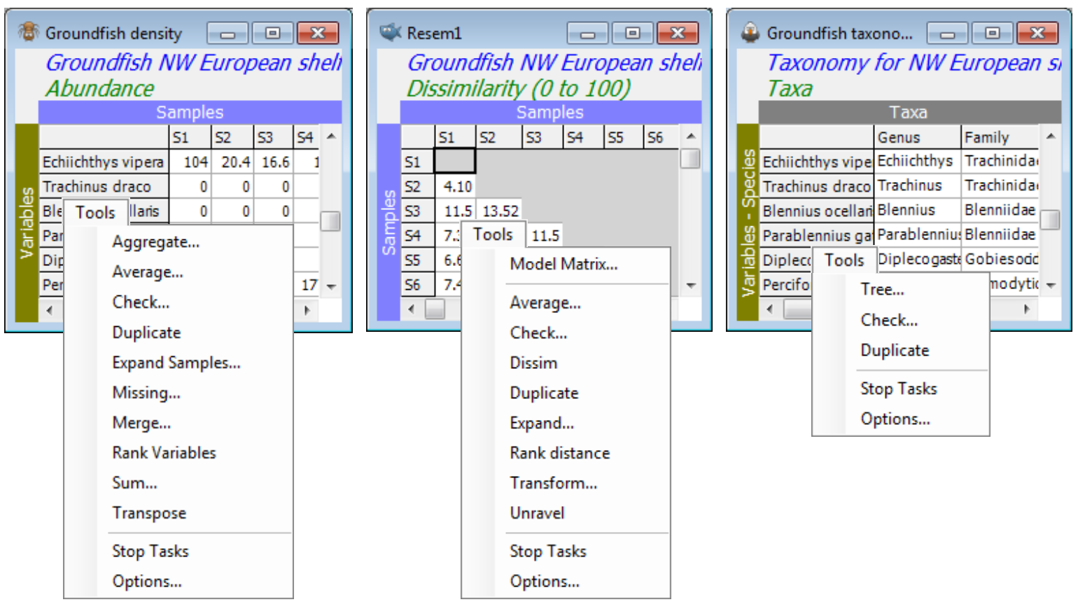
Close any open workspace and open Groundfish ws, last seen in Sections 7 and 6, demonstrating cluster analysis. If not available, open the data file Groundfish density in directory C:\Examples v7\ Europe\Groundfish, of species counts from 277 samples in 9 sea areas of the NW European shelf (factor area), and also the variable information file Groundfish taxonomy, defining the Linnaean taxonomy of genera, families, orders and classes for the 93 groundfish species monitored. Create a resemblance matrix (Resem1) in any way you like. Now compare the choices on the Tools menu when the active window is a data, resemblance or variable information sheet.
The section works through the choices in (very roughly) alphabetic order, with a few transpositions where menu items or data sets are better exemplified in combination. One or two more specialised routines will be deferred until they are needed (e.g. Tools>Expand in Section 14) and the Average (and Sum) options have been met sufficiently often in previous pages only to need an initial recap.
Average and Sum on data matrices; Average on resemblance matrices
Tools>Average and Sum operate in the same way on data sheets. For example, when (Samples• Averages for factor: area) & (Variables•No averaging) is selected, they average (or sum) across all samples with the same level of the specified factor, separately for each variable (species), here creating a derived data sheet of averaged (or totalled) communities for each area, which can be input into the same multivariate analysis options as the original matrix. Averages are taken for the specified factor not across it), e.g. if the above set of 277 locations (identified by a factor site) had been sampled at several times, then Tools>Average for factor site gives time-averaged site means. All factors in the original matrix are taken across to the new sheet, and factors such as area would still be well-defined over the 277 sites. (However, if the averaging had been for times, across all the sites, then the area column in the Factor sheet would consist only of Undefined! entries, since the averaging has mixed different areas). If the number of sites in each of the 9 areas is balanced then Average and Sum leads to the same ordination because the sheets differ only by a constant factor – most resemblance measures are unaltered by an overall scale change. If replication is unbalanced, however, then it is unwise to use Sum, because the outcome (using Bray-Curtis at least) would be sensitive to the different total abundances from the differing group sizes – Average is preferable.
A less common option is, for example, Tools>Sum>(Samples•No summing) & (Variables•Sums for indicator: class#) which would retain all 277 samples but total the matrix over the species to give just two new variables, class 1 (Chondrichthyes) and 2 (Osteichthyes). Pooling abundances to higher taxonomic levels is quite a common requirement but this is more naturally achieved with the Tools>Aggregate routine, discussed below. It is possible to Sum (or Average, though that is very unlikely) on both the axes, e.g. (Samples•Sums for factor: area) & (Variables•Sums for indicator: class#) would give a 2$\times$9 sheet of totals of each of the 2 classes in each of the 9 areas.
The main difference between Tools>Average or Sum and the Analyse>Summary Stats routine, new in PRIMER 7, is that the former computes means or sums within groups of samples (and/or variables) whereas Summary Stats will calculate these (and several other) summary statistics only over the full set of samples or variables (and in succession, not both at once, if both are required).
In PRIMER 7, the averaging facility extends to resemblance matrices: Tools>Average>(Factor/ indicator for groups: area) takes the average, e.g. for area 1 and 2, of all resemblances between pairs of samples, the first in area 1 and the second in area 2. It does this for all pairs of areas, thus giving a (9 $\times$ 9) triangular matrix of area resemblances. (These are the values at the head of each SIMPER table, defining dissimilarities between pairs of groups, which are then broken down into species contributions, Section 10 – but they are now more conveniently held in resemblance form). As the dialog implies, the averaging could also take place on variable resemblances, if groups are defined over those – perhaps coherent species groups from Type 3 SIMPROF tests (Section 10).
Aggregation
So far we have only seen variable information sheets, containing taxonomic (or other) hierarchies (*.agg files), used in calculating specialised forms of resemblance which exploit the relatedness of species in the samples being compared (Section 5). More significantly, this idea of relatedness or distinctness, as expressed in the variable information of the whole taxonomic tree, is the basis of a suite of biodiversity measures (Section 15). But the nomenclature of aggregation file (*.agg) comes from the original use of such taxonomies simply to aggregate up an abundance (or other) species matrix to, for example, genus level, i.e. to create a matrix of the abundances that would have been recorded had the species only been identified to a coarser taxonomic accuracy. There are several reasons for wishing to do this, e.g. the taxa might be thought too prone to mis-identification at the species level. Perhaps the data matrix was created over time by several taxonomists with differing expertise in particular taxonomic groups – a ‘lowest common denominator’ taxonomic level would then certainly lead to a more robust multivariate analysis. Alternatively, the motivation might be resource-driven – if it is possible to establish a putative environmental impact through community change just as clearly with a family-level as a species-level analysis then routine monitoring for that type of impact might be more cost-effectively carried out with data identified to the coarser level. Chapter 10 of CiMC gives many practical comparisons of species- and higher-level analyses.
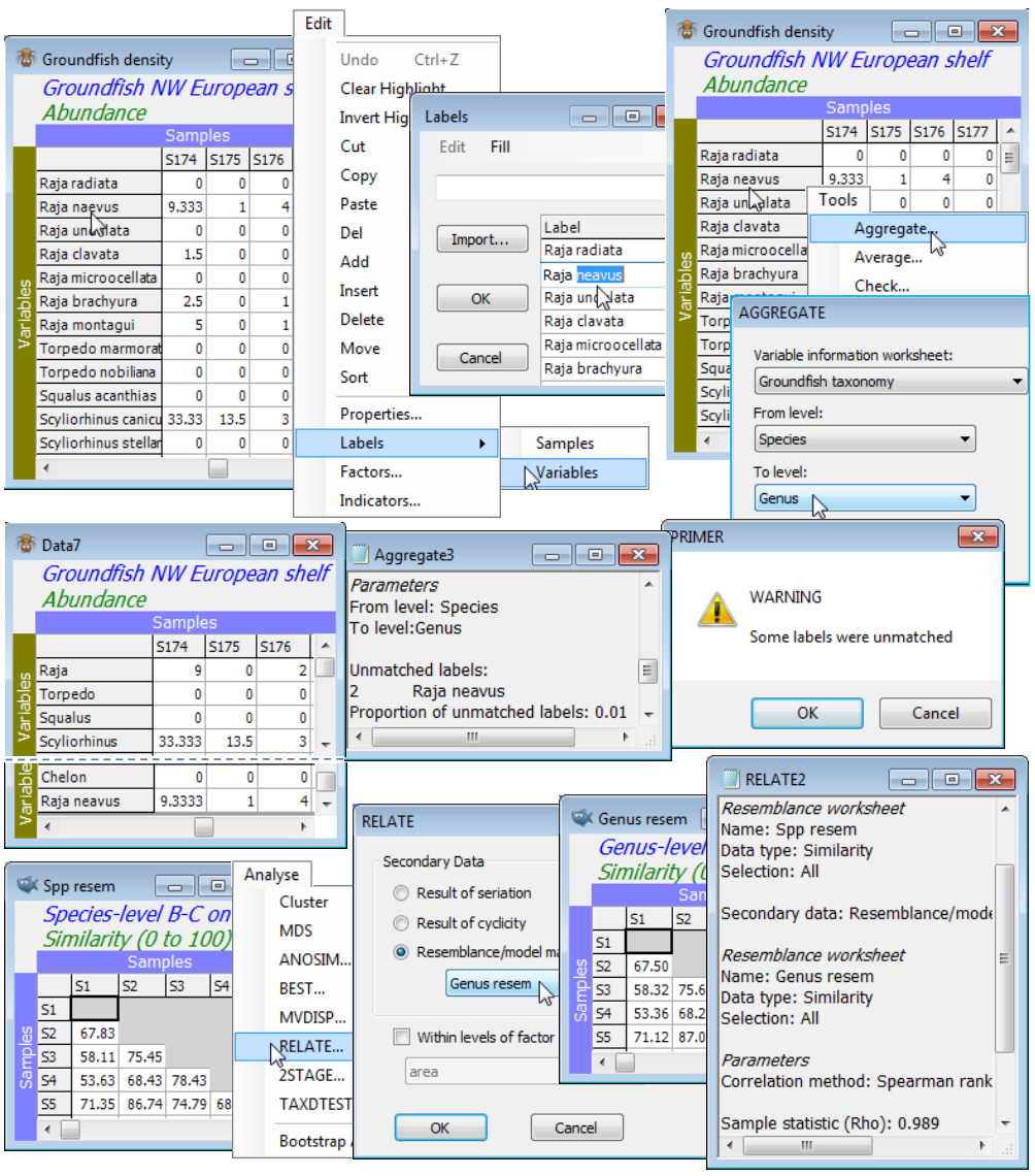
Whilst, as noted above, pooling the entries for species subsets, separately for each sample, could be accomplished by setting up an indicator and using Tools>Sum, this is more conveniently carried out with Tools>Aggregate. This works on the original data sheet (prior to any transformation) and specifies a variable information (aggregation) sheet and the hierarchical levels between which the aggregation needs to take place. Of course, unlike data and resemblance matrices the aggregation sheet is not restricted to numeric entries – its variable labels will typically be full species binomial names, and the subsequent columns the increasingly higher level (genus, family, order etc) names. The advantage of pooling using Aggregate is that the variable information file of the taxonomic (or other) hierarchy can be a look-up table which applies to a wide range of different data sets. There is no necessity for it to have the same number of species, or for those species to be in the same order, as in the data matrix, as long as all the data matrix species can be found in the more comprehensive faunal list which constitutes the aggregation sheet. Correct (or at least consistent!) spelling is thus essential, including spaces, periods etc. If a species name is not found, a warning is displayed, the results window lists which names were not matched, and these species are retained – with the same values – and with their species name being the higher-level variable name in the aggregated matrix.
Groundfish density and Groundfish taxonomy should be open in the current workspace. In this case the two sheets have the same full list of 93 species in the same order. With Groundfish density as the active window, Tools>Aggregate>(Variable information worksheet: Groundfish taxonomy) & (From level: Species) & (To level: Genus), pools the densities to a sheet which you should rename Groundfish genera. Square-root transform both data sheets and compute Bray-Curtis similarities. There is little point in trying to compare the nMDS ordinations for the two cases since the large number of samples (277) makes 2- (or 3-d) representations inadequate (high stress). But Sections 13 & 14 make much use of the idea of non-parametric correlation of resemblance matrices, e.g. with the Analyse>RELATE routine giving a measure of agreement in representation of sample relationships. Running this on the species and genus similarities gives a high level of agreement, $\rho$=0.989. You might like to start the example by mis-spelling a species name (e.g. Raja neavus) to observe the consequences, then change it back before running the comparison.
Check on aggregation files
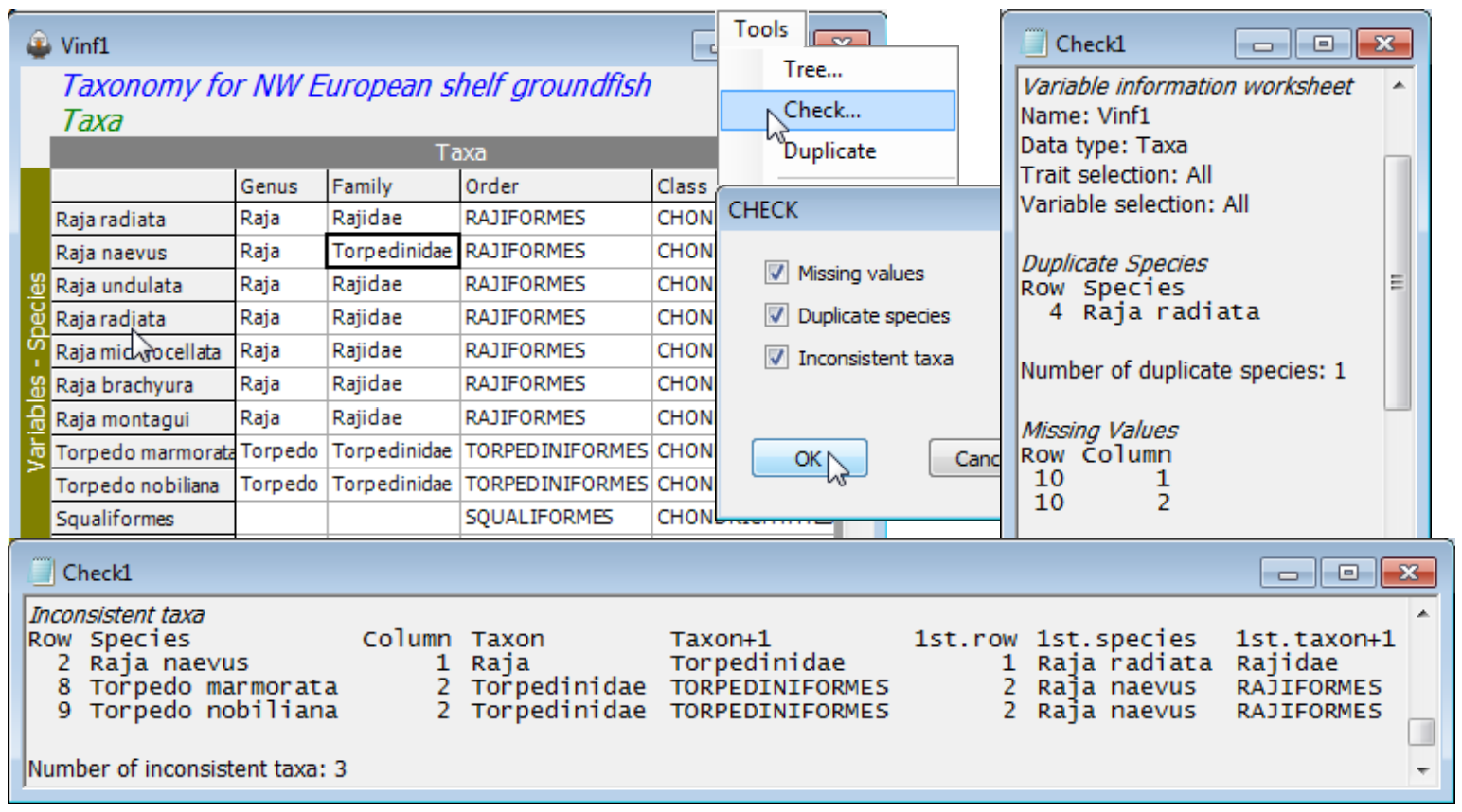
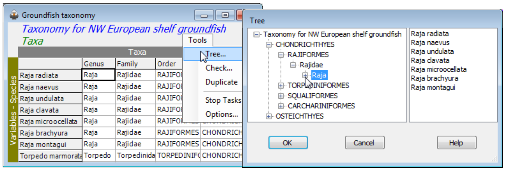
Use the open aggregation file, Groundfish taxonomy, to show the smaller set of Tools items (Tree, Check, Duplicate) available when the active window is of variable information. Tools>Duplicate has been seen previously for worksheets and plots (in Sections 3 and 8). Here it has the same effect, taking a copy of the Groundfish taxonomy window, called Vinf1, to the head of a fresh branch in the Explorer tree. Insert the following errors in Vinf1 to demonstrate the Tools>Check option:
a) overwrite Raja clavata (row 4) in the Species column with Raja radiata (by taking Edit>Labels>Variables and double clicking in the Raja clavata label and typing in the incorrect name);
b) whilst in the Labels dialog change Squalus acanthias (row 10) to Squaliformes (note that upper or lower case does not make a difference when matching names), and OK to exit back to the Vinf1 sheet, then delete Squalus and Squalidae from the genus and family name for that taxon;
c) change Rajidae to Torpedinidae as the family name for Raja naevus (row 2).
(Note that the row/column numbers of an entry can be found by clicking on it – the status bar at the bottom right displays the current cursor position). Then Tools>Check finds three types or error:
-
Duplicate Species in row 4 (the repeat of Raja radiata) – labels (samples or variables) should always be unique in a PRIMER worksheet, otherwise matching conflicts can easily result;
-
Missing Values (blanks) in row 10. This represents a common situation where only coarser-scale identifications can be made for some taxa. Nonetheless, aggregation sheets need to be complete, in order to avoid incorrect matching. E.g. another species from a completely different order but with a blank family (and genus) entry would be pooled with the Squaliformes abundance when the matrix is aggregated to genus or family level, because both entries have the same (blank) family name. Similar problems would occur with taxonomic distinctness calculations (Section 15). So blank entries should be filled with the names from the immediate right or left, depending on the context (often it make sense to fill from right to left). Here put Squaliformes in the two blanks – the routine does not object to the same name being used in different taxonomic levels.
-
Inconsistent taxa in rows 2, 8 and 9. In fact there is only one mistake, the family identification of Raja naevus, picked up in the correct row (2) because Raja has been established by row 1 to be a genus name in the Rajidae family, thus cannot also be a genus name in the family Torpedinidae. Quite often, however, an error is not discovered until a conflict occurs much later in the sheet, on a row which may be correct. This is seen in the inconsistent identification of the two Torpedo genera though neither are wrong. PRIMER 7 has greatly improved its diagnostics here, by listing not just the row and column on which the conflict occurred (in the first 5 columns of the output: row, species name, column, entry in that column, entry in the following column) but also what the conflict with an earlier row was (in the final three columns of the output: the earlier row, its species name, the entry in the earlier row causing the current conflict). So, Torpedo marmorata (row 8) in family Torpedinidae cannot be in order Torpediniformes because in a previous row (it identifies row 2) the family Torpedinidae were given as in order Rajiformes. With this level of diagnostics, errors in aggregation files (they commonly occur!) should be more easily fixed.
Tree menu; Check on datasheets & resemblances; Undefined resemblances
The other Tools menu item for aggregation sheets is distinctive to this case, namely Tools>Tree; it simply displays the hierarchical structure of an aggregation file in the same way as the Explorer tree, in a left-hand panel. Successive clicking on the  icons unroll the taxonomic structure, and it can be rolled back with
  . No operations can be performed on the display in this state.
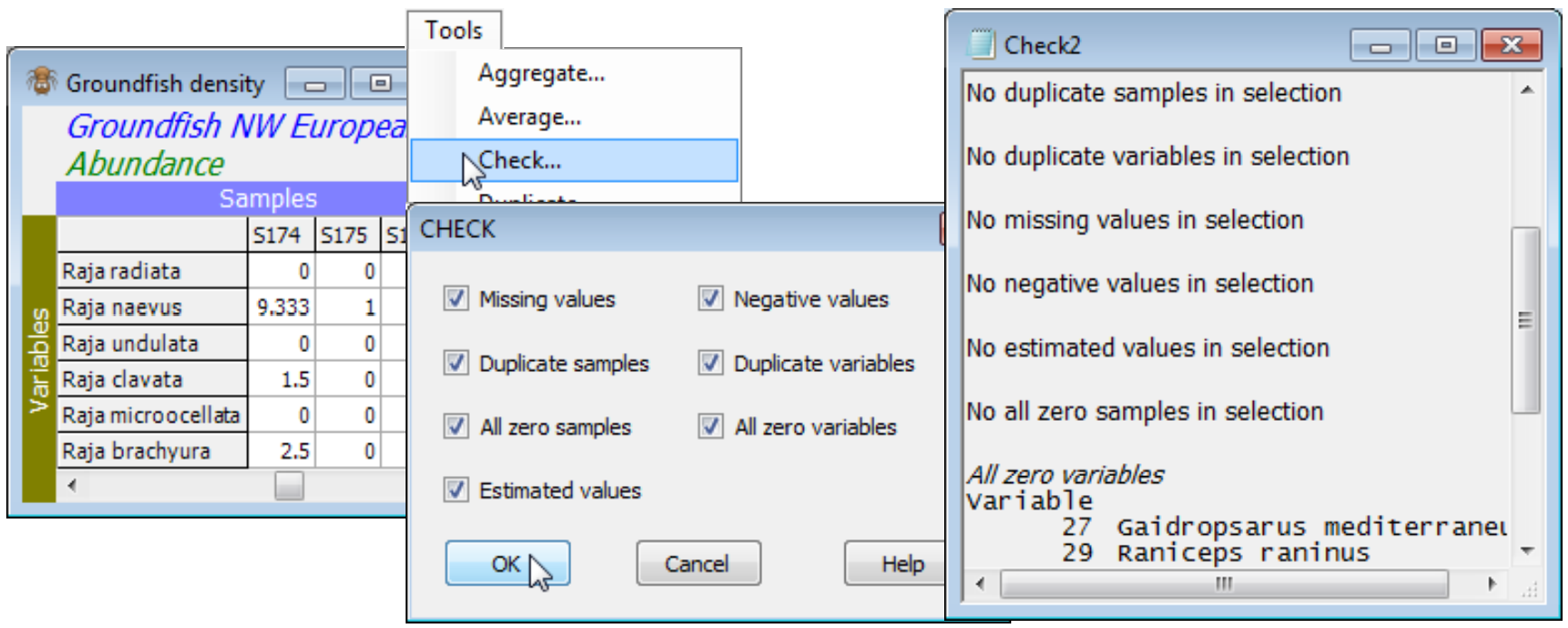
When the active window is a datasheet, Tools>Check can check for the following: a) ✓Missing values, identified in the sheet by ‘Missing!’, and which might have been read in as blank cells in an Excel worksheet for example; b) ✓Negative values, which are not appropriate for abundance-type data analysed by Bray-Curtis, though common for environmental variables (especially normalised) input to Euclidean distance; c) ✓Duplicate sample (and/or) variable labels, which are tolerated for some analyses (warnings are usually given) but are best avoided wherever possible; d) ✓All zero samples (and/or) variables; and e) ✓Estimated values, displayed in red type in the matrix. The latter come from applying Tools>Missing (seen shortly) to environmental variables – or to other normally distributed data – containing Missing! cells, which otherwise might not be tolerated by some analysis routines requiring complete data. All or any of the 7 boxes can be ticked. Whether it is important to check for a particular attribute depends on the analysis. For example, species which are zero over all samples will be ignored when Bray-Curtis similarity is computed among samples, and can safely be left in the matrix, but all-zero samples are potentially more of a problem since Bray-Curtis similarity between two blank samples is set to ‘Undefined!’. Dependent on the context, these samples might best be omitted, or a different similarity used (e.g. zero-adjusted Bray-Curtis, Section 5), or the entry left as ‘Undefined!’, i.e. treated as unknown.
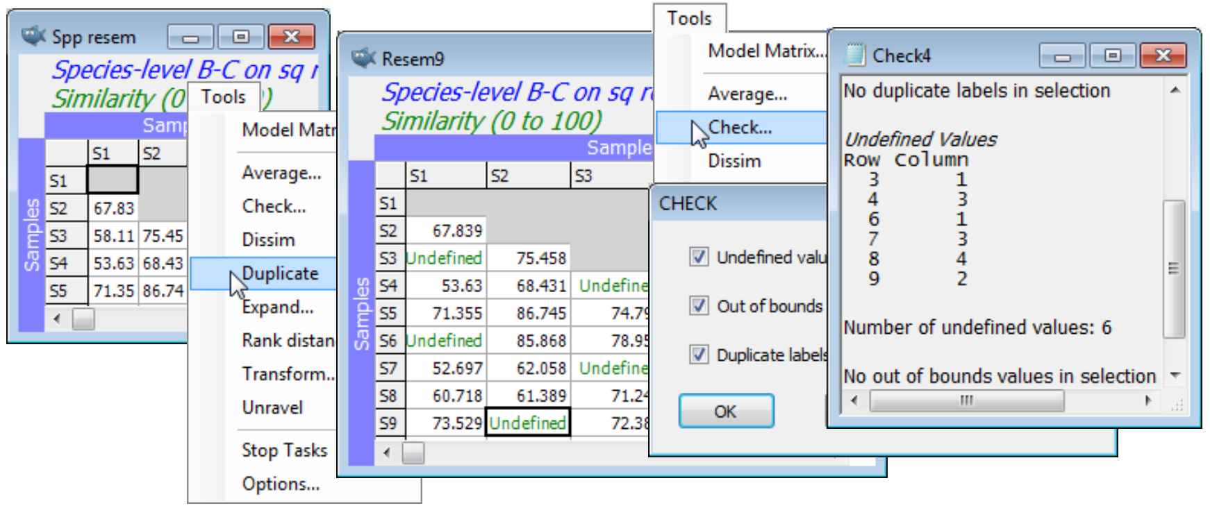
When the active window is a resemblance sheet, Tools>Check looks for only three data attributes: a) ✓Undefined values, arising as suggested above; b) ✓Out of bounds values, for distance coeff-icients (or transformations) that return very large or small values (NaN); and c) ✓Duplicate labels, as above. Blanking a cell in a resemblance matrix sets it to Undefined! status, and several of the core routines using resemblances (e.g. MDS, Cluster, ANOSIM) are carefully written in PRIMER to tolerate a few Undefined! entries, treating them as unknown. (You can appreciate that knowing the similarities $S_{12}$, $S_{13}$, $S_{14}$, $S_{23}$, $S_{24}$ might enable you to place four samples in relation to each other without knowing similarity $S_{34}$). Blanking out NaN (Not a Number) entries, to Undefined!, is one possibility therefore, but others may be equally good or better (replacing by a large, but finite value, modifying the coefficient or transformation which generated them etc).
Duplicate; Merge (/join) operations
Tools>Duplicate operates in the same way whether the active window is a data array, resemblance matrix, variable information sheet or plot. In the case of a Graph window, Duplicate is the only specific option offered on the Tools menu, and there are no choices at all for results windows (since they are not capable of amendment once written) except for the Stop Tasks and Options items which are available on the Tools menu whatever the active window. Unless the window is at the top level of a branch already – as a variable information (aggregation) file will always be – an option is offered of (•On existing branch) or (•Start new branch), so that the original links to other sheets and factors can either be retained or a fresh start made. On a new branch, any subsequent amendments to factors, for example, will not then carry back to the originally linked sheets (unless specifically imported by them, with Edit>Factors>Import).
On the above resemblance matrix Spp resem for the Groundfish data, take Tools>Duplicate>(•Start new branch) and, in the copy, blank out entries at random. A run of Tools>Check picks up those now Undefined! entries, but MDS will accept the matrix in this form and produce a plot probably very similar to an MDS run on the intact matrix. Save and close Groundfish ws.
(Tasmanian meiofauna)
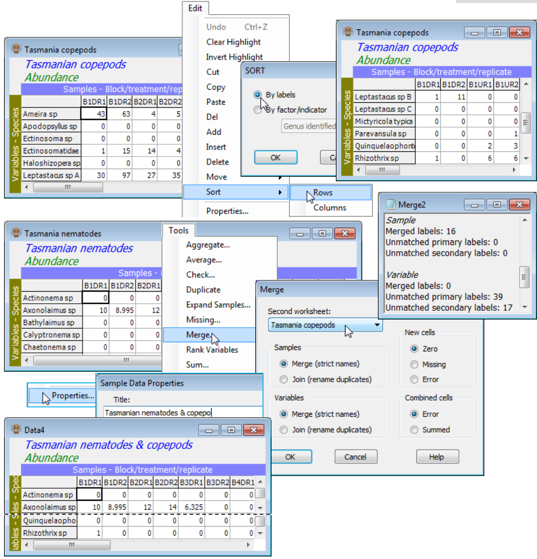
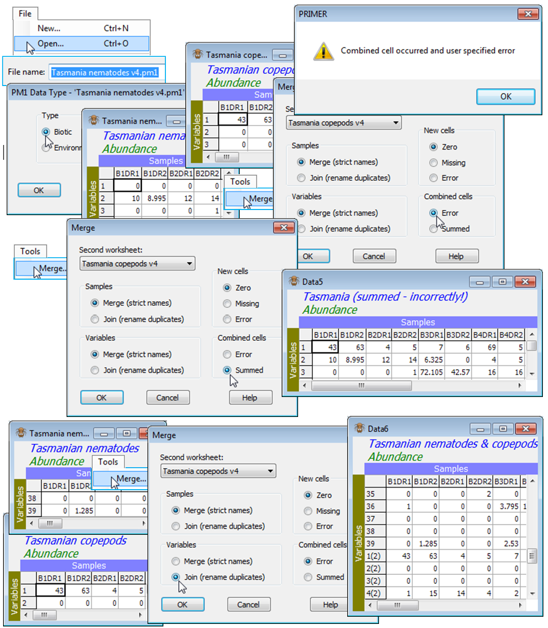
The nematode and copepod datasheets from 16 samples at a Tasmanian sand-flat (C:\Examples v7\ Tasmania meiofauna) were seen in both the previous two sections, in workspace Tasmania ws, but if the latter is not available open Tasmania nematodes and Tasmania copepods in a new workspace. With Tasmania nematodes as the active window, run Tools>Merge>(Second worksheet: Tasmania copepods)&(Samples•Merge(strict names))&(Variables•Merge (strict names))&(New cells•Zero) &(Combined cells•Error), i.e. all the default options. The latter two options of new or combined cells do not come into play here, but are discussed later. The resulting merged datasheet now has 56 rows (the 39 nematode species then the 17 copepods). The results window shows that all the samples matched (and the species did not) in the way expected. The title for the new sheet is taken from the first (active) window, so to avoid confusion should be changed using Edit>Properties.
Now, re-order the columns in Tasmania copepods by Edit>Sort>Columns>(•By labels), sorting the samples in a different (alphabetic) order for the copepod matrix of B1DR1, B1DR2, B1UR1, B1UR2, … than the nematode sample order of B1DR1, B1DR2, B2DR1, B2DR2, …. Nonetheless, a re-run of Tools>Merge with Tasmania nematodes as the active window, and with exactly the same options, will result in a merged datasheet identical to the previous one, the ordering of samples having been taken from the first (active) window.
Combined cells in Merge
Occasionally, use of strict label names does not give the this desired outcome, and the default behaviour can be changed to force PRIMER to consider an identical label, but in a different matrix, to be treated as a different name. For example, this might be needed when species names have not been provided for either set, and the variable labels are just the numbers 1, 2, 3, …. Species 1 in the first set is not to be taken as the same variable as species 1 in the second set, and the default options in Merge will cause difficulty in this case. Equally possible is the opposite case where the species names match in the two matrices, but the same sample labels are repeated, though should not be equated. Samples collected in year 1 might be labelled by their site identification. A second matrix of data from those sites in year 2 might use exactly the same set of sample labels, i.e. without reference to the year. This causes no confusion if the matrices are to be analysed separately, but a Merge under the default of strict name-matching would place the two matrices on top of each other (because they have exactly the same row and column labels!). The two options given in such a case are (Combined cells•Summed) or (Combined cells•Error). The first literally adds the two matrices, element by element. Very often though, this is not the desired behaviour, so the default is the second option: if a Merge instruction results in an attempt to combine two cells, an error results.
In the same workspace, take File>Open on the data files Tasmania nematodes v4 and Tasmania copepods v4 (in *.pm1 format, from the old DOS-based PRIMER4), which should be read in as Type•Biotic. These are the same nematode and copepod matrices as their *.pri counterparts except that PRIMER v4 held species lists as separate files so both the *.pm1 files have variables numbered just 1, 2, 3, …, though the species are different in the two matrices. A Tools>Merge on them, with the default of (Variables•Merge (strict names)) will potentially give combined cells. Try this with both (Combined cells•Error) in place, to note the error message and the fact that execution then stops. Then repeat with (Combined cells•Summed) – those cells with the same species and sample numbers are then simply added together. This may occasionally be a useful option, e.g. it would allow for easy collation of data for the same samples by several different observers (though it must be debatable whether such a piecemeal approach to data matrix construction – losing information on potential observer differences – is often desirable). Taking nematode species 1 to be the same taxon as copepod species 1 and adding the two counts is clearly nonsense in this context, however. The solution, if it is easier to join the arrays in PRIMER and then rename the variable labels later, is next described (the Join option) – this forces the arrays to be placed one after the other.
Avoiding strict label matching
The best policy to avoid confusion is to use precise, unique species and sample labels (typically, the sample label would be a conglomeration of all the different study design factors and a replicate number). However, conflicting desirable criteria can sometimes arise, e.g. when the pattern of sites from year 1 is to be compared with the pattern in year 2, using the RELATE test (Section 14) on the two separate similarity matrices, identical sample (site) labels are ideally needed in both arrays, so they can be matched. But, as just pointed out, a Merge of the two data sheets underlying these similarities (so that both year 1 and 2 sites can be seen on the same nMDS say) requires the sample labels to be different. Thus, PRIMER is not dogmatic about label matching: several routines, which include Merge and RELATE, are able to ‘fudge’ the matching and provide a natural alternative. In Merge, this is shown above, using the •Join (rename duplicates) option, used either for Samples or Variables (or possibly both, to create a block diagonal matrix, though this is unlikely to be needed). For Tasmania nematodes v4 and Tasmania copepods v4 sheets to be placed one under the other, even though they share species labels, take Tools>Merge>(Variables•Join(rename duplicates)) and defaults for the other options, i.e. (Samples•Merge(strict names)), and there should be no combined or new cells. The copepods are labelled 1(2), 2(2), …, to distinguish them from nematodes 1, 2, … Save the workspace Tasmania ws and close it.
Merging non-uniform species lists; (Phuket coral reefs); (Clyde dump-ground study)
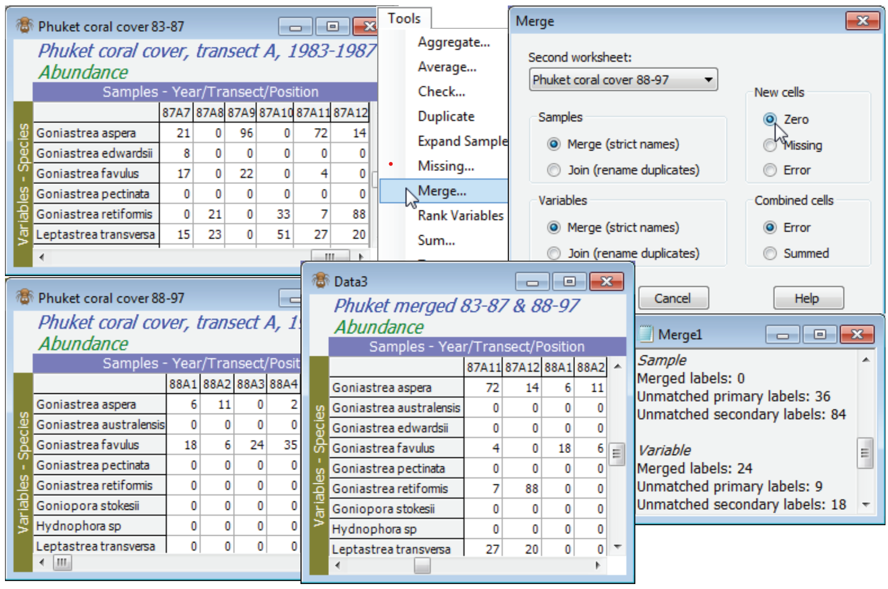
Perhaps the greatest benefit of the strict label matching in PRIMER is the ability to Tools>Merge assemblage data when two sets of samples, taken at different times or places, are not recorded on a common data sheet, with predetermined taxonomic categories. Species names, or other operational taxonomic units, must be consistently spelt (even to spaces) in the separate lists, so that the strict matching of variable names can take place. But there is then no necessity that the two sheets hold the same set of species, in the same order. Typically, lists will be of different length, with some species in each list not appearing in the other. Using (•Merge (strict names)) copes automatically with this, filling any spaces created in the merged array either with (New cells•Zero), relevant for assemblage-type data, or with (New cells•Missing), more appropriate for environmental variables. A third option (New cells•Error) stops the procedure with an error message if any new cells are created. This can be a useful safeguard if the intention was to join two data sheets with exactly the same set of variables – an error alerts you to the fact that there may be variable names misspelt.
The Ko Phuket coral reef assemblage data was introduced in Section 8 and the workspace Phuket ws last seen in Section 9. In each sampling year, 12 plotless line-samples were taken along a fixed onshore-offshore transect (A) and area cover determined of each coral taxon. From the directory C:\Examples v7\Phuket corals you will need to have open the three *.pri files of data for different runs of sampling years: Phuket coral cover 83-87, 88-97 and 98-00,only the first two of which were opened in earlier sections. (The early years straddle sedimentation impact from dredging operations for a new deep-water port, 1986/7, and the later ones a sustained Indian Ocean high pressure period with desiccation from lowered sea levels, 1998, with a more stable environment in between). Note the different (but overlapping) species lists of these three sheets. With the active matrix of 83-87, Merge this with 88-97, and merge the result again with 98-00, choosing zeros for the new cells, and tidying up the new sheet appropriately (e.g. renaming the window, amending the title with Edit>Properties and sorting the species in the merged sheet with Edit>Sort>Rows>•By labels).
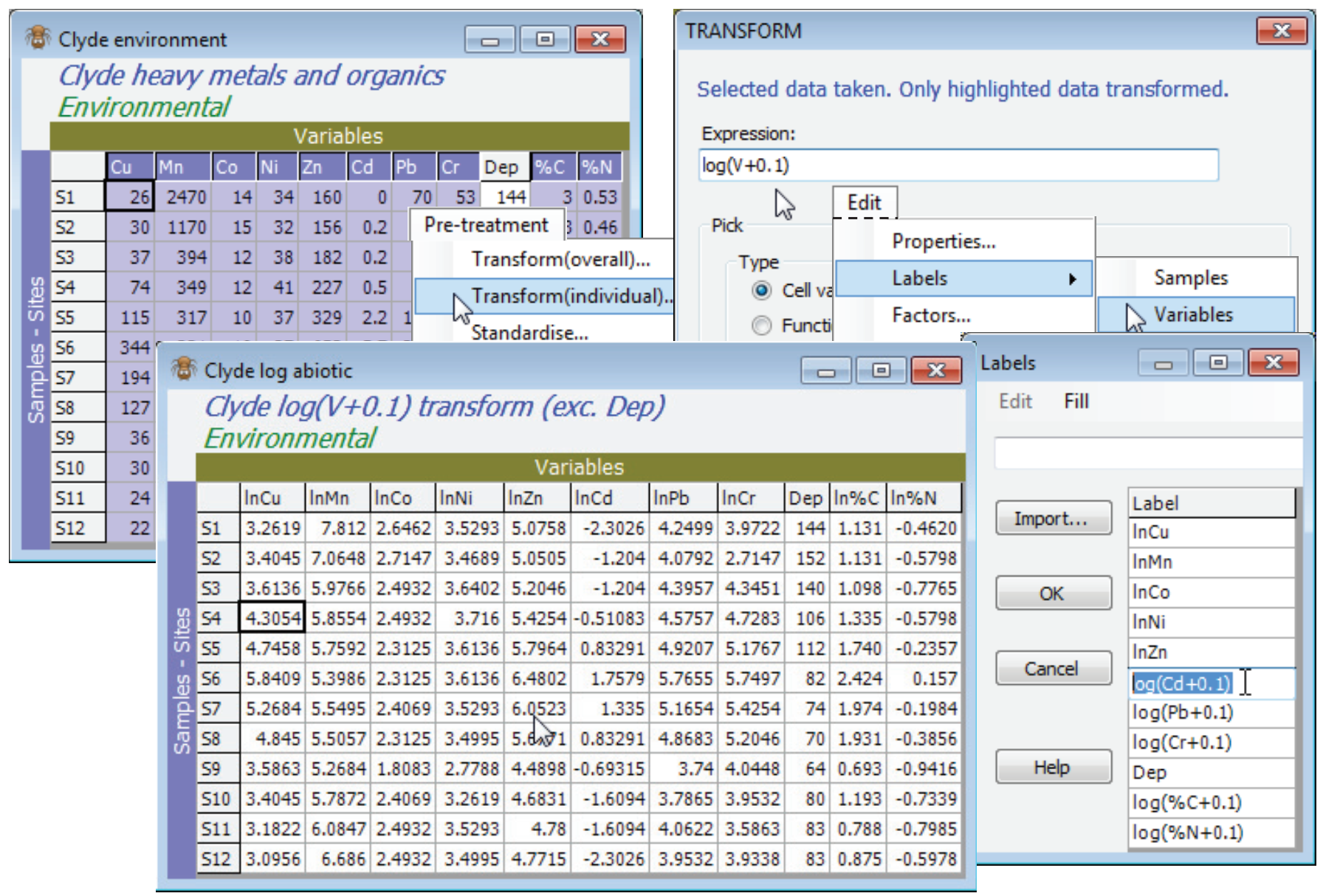
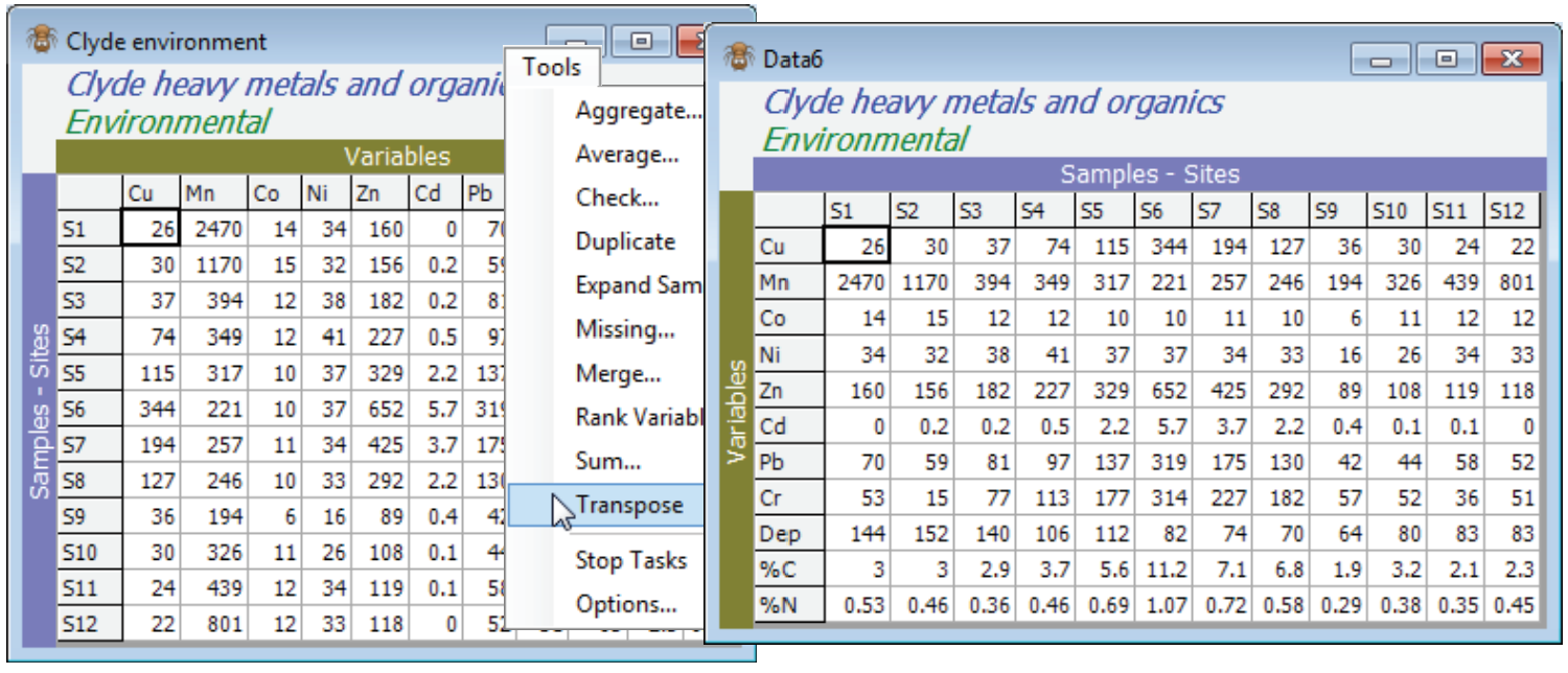
Save and close the workspace (Phuket ws), and from C:\Examples v7\Clyde macrofauna open Clyde environment, of 11 abiotic sediment variables (Cu, Mn, Co, Ni, Zn, Cd, Pb, Cr and %carbon and %nitrogen, plus water depth) sampled in 1983 at each of 12 sites (S1 to S12) along an E-W transect across the Garroch Head sludge dump-ground in the Firth of Clyde – see Fig. 1.5 of CiMC (data from Pearson TH, Blackstock J, 1984 Dunstaffnage Lab Report, Oban, Scotland). We will use these data (seen often in CiMC) for the rest of this section and most of the next one.
Missing data estimation
The subject of missing data has arisen several times already (Sections 1, 3, 5) and the point made that the terminology and sheet entry Missing! refers only to variables (usually environmental -type variables) that are not recorded for some samples. It does not refer to designs which were intended to be balanced but for which some replicate samples were not analysed for some reason, over all variables. (Unbalanced replication is not generally a problem to handle in PRIMER, since balance is not required for most of the testing that PRIMER, and PERMANOVA+, are able to carry out.)
Some of the routines, including PCA (next section), require the user to enter a complete matrix, with no missing values. At a simple level, it is fairly clear why this should be so. For the trivial 2-variable case in which PCA was introduced in Chapter 4 of CiMC, imagine losing one variable value for one of the samples. What is now that sample’s contribution to total variance? How can it be projected perpendicularly to the best-fitting line through the points? How can that first PC axis be determined at all without knowing the contribution of this sample, and so on? In fact, a solution to this was suggested in Section 5 when discussing computation of resemblance measures in the presence of missing entries – it is possible to adjust Euclidean distances, or any other distance/ dissimilarity measure, for the crude bias that may come (and certainly will come for Euclidean distance) from some pairs of samples having more matching variables across the two samples than others do. The resulting (near-)Euclidean resemblance matrix is then complete and a choice can be made between MDS (possibly metric) or PCO in the PERMANOVA+ add-on software. The latter is a PCA when the matrix is Euclidean (though the missing data will make that identity not quite true). An alternative is to remove (listwise) as few variables and samples as possible, in a judicious balance, such that a complete matrix is left. The routines Tools>Check, Select>Samples>(•No missing values) or Select>Variables>(•No missing values) will help with this. When there are large blocks of missing data – a subset of the variables were simply not recorded at a large group of sites – then this is likely to be the most realistic option. In other situations, where there is very little missing data, it can seem very wasteful of valuable resources – a whole sample would have to be deleted because one variable is missing, or a whole variable deleted because it was not measured for one sample. In this case, there are then two realistic options – work always from a resemblance matrix and allow PRIMER to adjust automatically the pairwise distances for the crude bias, or use a completed data matrix obtained by estimating the missing values with the EM algorithm. If some restrictive distributional assumptions apply (with rather few missing values and good correlations between some of the variables), this can provide a less crude adjustment and should be attempted.
EM algorithm assumptions
Tools>Missing is designed to operate only on matrices for which: a) assumptions of multivariate normality can be made; b) there are many fewer variables than samples, so that there are enough data values to be able to estimate the parameters representing means, variances and correlations of all the variables, with reasonable stability; c) there are rather few missing data points (each of those is a new parameter that needs estimating also); d) the data points are thought of as ‘missing at random’, rather than missing because they were so extreme that they could not be recorded; e) the samples are treated as of unstructured design, rather than, for example, utilising information about their status as replicates from a set of a priori defined groups.
Many of these are the assumptions that the methods of PRIMER are trying to get away from, of course! But that is mainly because they are completely impossible to satisfy for assemblage data; they may be much more realistic for continuous, environmental-type data (including, for example, morphometric variables). The estimation technique that PRIMER uses is the standard statistical method under these conditions, namely the EM (expectation-maximisation) algorithm. It is rather tricky (and dangerous!) to give guidelines for when the method will prove acceptable, but you do have some help from the algorithm. Firstly, if you set it an impossible problem (far too many parameters to estimate for the number of data points you have) then it will fail a convergence threshold and display an error message (max number of iterations exceeded). Secondly, when it does converge, it is also able to provide an approximate standard deviation for its estimate of each missing value. If this is large then there has clearly been insufficient information to pin down a likely value for the missing cell. As a rough rule-of-thumb, you should not expect to be estimating more than about 5% of your data points if your analysis is to retain any credibility(!), and you should have enough samples n compared with (selected) variables p and missing cells m, so that there is a half-decent number of data points per estimated parameter $DpP = n/[(p+3)/2 + (m/p)]$ (around 7 is sometimes cited, in general contexts). When this criterion is far from being met using the whole matrix, you may be able to take a piecemeal approach, selecting just a small set of the most relevant variables to drastically reduce p. The method is clearly only going to provide you with something useful if there are variables that correlate fairly well with the one containing the missing data, so that it has some basis for the prediction. Draftsman Plot will work on datasheets with missing cells, so you can use this (and its correlation table) to select out good subsets of variables for estimating each missing data cell. Use of Tools>Missing should not be seen as an automatic process therefore – you must expect to have to work hard to justify any data points that you are making up! In the end, common sense is the best guide here, as always. Look at each estimated value – they are always displayed in the worksheet in red – and compare it with the range of values from the other samples for that variable. Does it look ‘reasonable’, or has something clearly gone wrong with the fitting routine? If all appears well, then it does have the objective credibility of being the maximum likelihood estimate of that cell, and not just some subjective value that you wish it was! Also, look at the standard deviation ($\sigma$) of the estimate in the results window and try sensitivity analysis. Add or subtract up to 2$\sigma$ from each of the estimated cell values at random, and re-run your PCA (or MDS, ANOSIM etc). Whatever you estimate for the missing values may make no difference to the outcome, if they are within a reasonable range of the other data – you then have a very credible analysis.
Missing data estimation (Clyde study)
Transformation options for the Clyde environmental matrix, Clyde environment, are discussed in more detail in the following (PCA) section, but the tool to carry out separate transforms on sets of variables, Pre-Treatment>Transform(individual), rather than transforming the whole array, Pre-treatment>Transform(overall), was met in Section 4, applied to the environmental data from the Ekofisk oil-field study. Here, all heavy metals and organics (10 of the 11 variables) will benefit from log transformation, to reduce their right-skewness and so bring these continuous variables closer to normality across the sites (in so far as that can be judged from only 12 samples!). Thus, highlight all variables except Water Depth (Dep) and take Pre-treatment>Transform(individual)>(Expression: log(V+0.1)) & (✓Rename variables), renaming the result Clyde log abiotic. Give the variables in this sheet shorter names (e.g. lnCu, lnMn etc) with Edit>Labels>Variables.
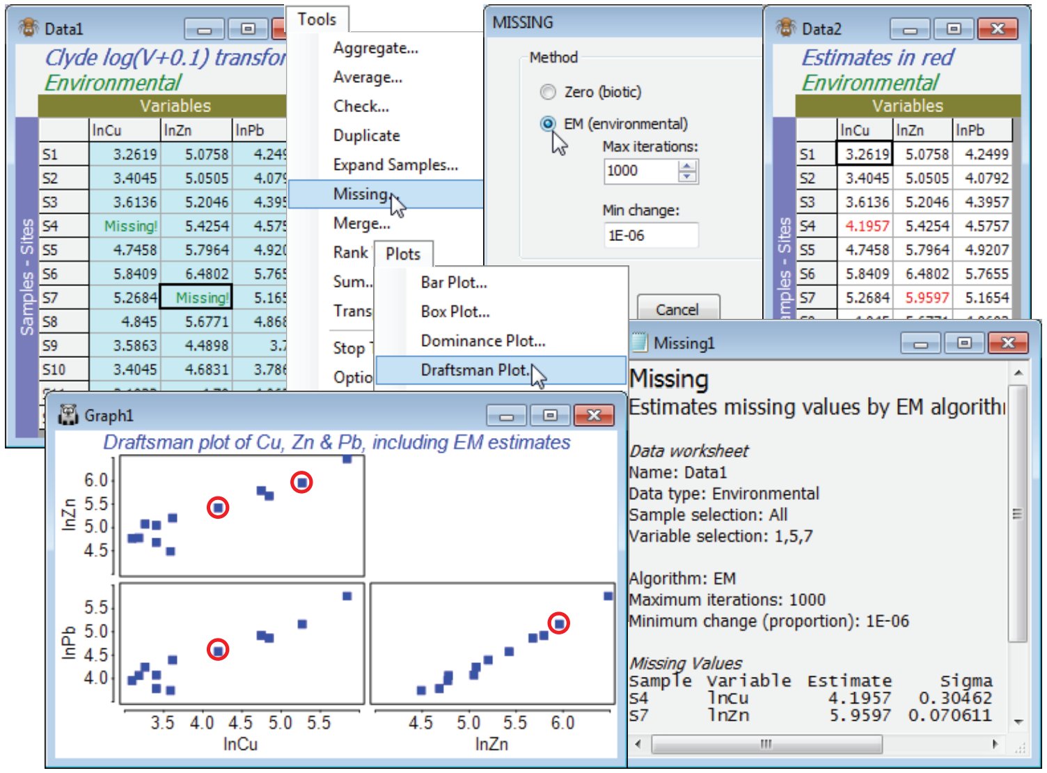
Take a copy with Tools>Duplicate and from this remove a couple of cells at random – perhaps (S4, lnCu) and hit the delete key, then (S7, lnPb) and delete again. Both cells will now be displayed as Missing!. Analyse>Draftsman Plot on this transformed data shows that normality assumptions are probably now acceptable (see the following section) but the above DpP criterion for the whole matrix fails badly (n = 12, p = 11, m = 2, so DpP = 1.7) and we should not trust the outcome even if Tools>Missing converges (it does not, here). The correlation matrix output with the drafts¬man plot does, however, show some very high correlations between e.g. Cu, Pb and Zn, which gives a better basis for prediction than the whole matrix. So, select just these three variables (highlight them then Select>Highlighted), and Tools>Missing produces credible missing data estimates of 4.18 (S4, ln Cu) and 5.26 (S7, ln Pb), compared with the original 4.31 and 5.17. Note that the ratio DpP = 3.3, which is still some way from respectability, but clearly is capable (sometimes at least) of producing useful results. The results window shows that the imprecision (under the assumption that the value is missing at random, of course) is lower for the estimated (S7, Pb) reading than the (S4, Cu) value, though both are rather well determined. The standard deviation of the estimate for (S7, Pb) is about 0.07 and for (S4, Cu) about 0.30, so that rough confidence intervals are (3.6, 4.8) and (5.8, 6.1) respectively. The reason for this difference in precision is clear from the draftsman plot for these three Cu, Zn, Pb variables, on which the respective points are manually circled (the plot window was copied and pasted to Powerpoint with Ctrl-C and Ctrl-V). The linear relationship between Pb and one of the other variables (Pb) is seen to be extremely tight, whereas Cu is not so highly correlated with either Zn or Pb, so there is inevitably greater uncertainty in the interpolation – it is a consequence of the multivariate normality condition that these relationships are estimated as straight lines. The estimates now need to be individually copied (click in the cell and Ctrl-C) and pasted back into the full matrix (Ctrl-V at the cursor). Of course the process is more automatic in less borderline cases, with larger n, when the full matrix can be input to Tools>Missing.
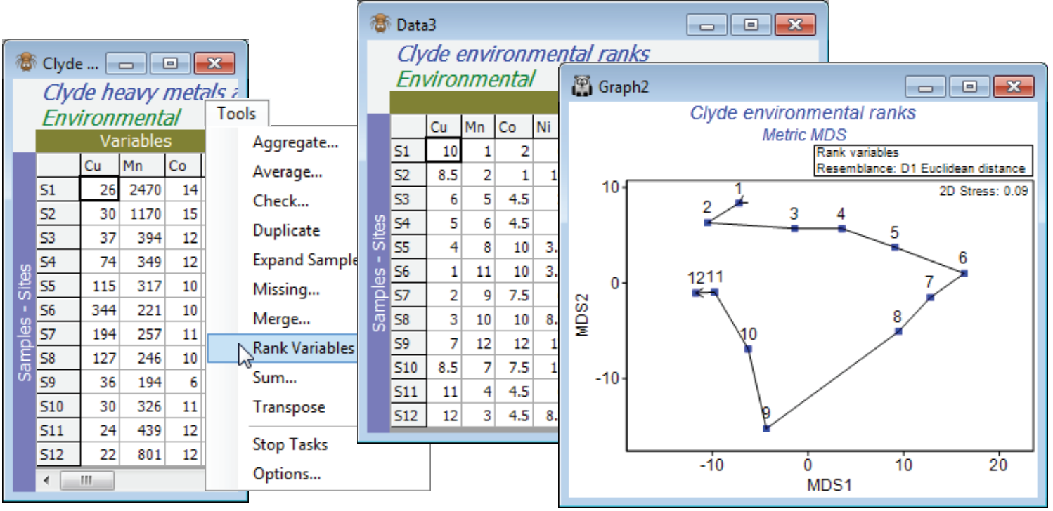
Ranked variables
The following section (on PCA) will discuss further the choice of particular transformations to avoid the sensitivity of PCA (and Euclidean distances in general) to outliers in some environmental variables, but choice of individual transformations is often a worry to practitioners. An alternative, eliminating the need for choice (but arguably losing some sensitivity in the ensuing analysis), is to replace variables by their ranks, namely the numbers 1, 2, 3, … for largest to smallest values across samples (modified if necessary to substitute average ranks for tied values). The main advantage is that the over-dominant contribution of outliers is automatically eliminated. For example, a variable whose values over the samples, in decreasing order, are: 25, 9, 7, 6, 6, 6, 4, 2, 2, 0 would generate ranks: 1, 2, 3, 5, 5, 5, 7, 8.5, 8.5, 10 respectively, and the effect is to make the outlying value of 25 no different than if it had been 15 or 10. Ranking each variable (separately) also removes the need for normalising the resulting array, which is needed (after transformation) with the usual approach, to ensure that all environmental variables take values across comparable ranges. Ranking places all variables on a common measurement scale, the numbers 1 to n (where n is the number of samples).
For the original (complete) Clyde environment sheet, take Tools>Rank variables and examine the outcome. Put this matrix through Analyse>Resemblance>(Measure•Euclidean distance) and then Analyse>MDS for a non-metric or metric MDS (the latter has a better chance of being acceptable because of the few points and the simple gradient structure, and importantly, the Euclidean distance matrix). In order to overlay a trajectory on the MDS with Graph>Special>Overlays>(✓Overlay trajectory)>(Trajectory numeric factor: Site#), you will need either to create the Site# factor for any sheet on the Clyde environment branch, with Edit>Factors>Add>(Add factor name: Site#), highlighting the column and Fill>Label number, to generate the values 1 to 12. (Alternatively, if you have already opened the abundance file Clyde macrofauna counts into the workspace, you can Factors>Import the factor Site# from that sheet). It is interesting to note the linearity of Shepard diagrams for both mMDS and nMDS but whilst the ordinations look very similar, the mMDS fit of a straight line through the origin is not quite such a good fit (stress = 0.09 c.f. nMDS stress = 0.03). The main point here, though, is that this ordination, based on ranked data, looks very similar to the PCA which we shall see in Section 12, based on transformation and normalisation of this data.
Ranked resemblances
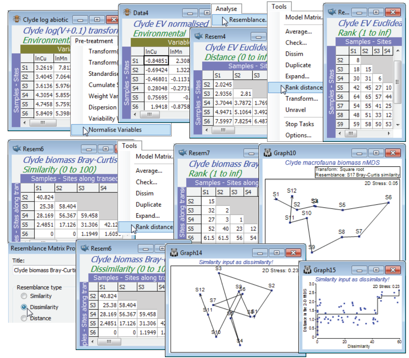
Ranking is also a menu option when the active sheet is a resemblance (Tools>Rank distance), but it operates a little differently. This time, all elements of the triangular matrix are ranked together, rather than separate ranking of the rows or columns of the rectangular data sheet. Do not get these two possible rankings confused! It is easy to fall into the trap of thinking that, because a ranked data matrix will be the same whether ranked from original or transformed data, if you are intending to rank the similarity matrix then initial transformation of the data does not matter. This is entirely wrong of course – ranking the similarity matrix is by no means the same as ranking the data then calculating the similarities! In fact, whilst ranking the data may play a marginally useful role for handling outliers in environmental matrices (as above), it rarely makes sense for assemblage data because it destroys the special nature of the (very many) zero responses, which would be assigned different tied ranks for different species. Ranking the resemblances, however, is rather central to the approach in PRIMER: many of the core routines (ANOSIM, RELATE, BEST, …) start from the ranked form of the similarity matrix, and nMDS ordination also exploits this rank order. For all routines, however, it is not necessary to enter the ranked form of the triangular matrix – if the result depends only on the ranks, this will be part of the internal calculation on the similarities. The menu item of Tools>Rank distance on a resemblance matrix is mainly here to help visualise and check the relatively simple computations underlying an ANOSIM test, for example (see the definition of the ANOSIM R statistic, a difference in mean rank dissimilarities, in equation 6.1 of CiMC).
For the Euclidean distance matrix from the above Clyde environmental data (transformed then normalised), take Tools>Rank distance to produce a rank resemblance matrix. Note that entries are just the numbers 1, 2, .., 66. Importantly, the convention PRIMER adopts here is always to return a distance-type matrix from the Rank distance operation, irrespective of whether it is given a similarity or dissimilarity/distance matrix (explaining why the menu item is called Tools>Rank distance). Thus rank 1 corresponds to samples (S11, S12), which are closest environmentally, and rank 66 to those furthest apart (S6, S9). To see this point about the direction in which ranks are assigned, open the macrofaunal biomass matrix for the 12 samples on the Clyde transect, Clyde macrofauna biomass, take a square transform and calculate Bray-Curtis similarity, as usual. Now take Tools>Rank distance on this similarity matrix and note that the resulting ranks again form a distance matrix, with the closest sites in assemblage terms (rank 1) being S3 and S4, and several pairs of sites tied on the largest, most distant rank (average of 61.5), namely S6 with S1, S2, S11, S12 etc, which are all pairs of sites with no species in common.
PRIMER handles its (distance) ranks in this slightly unconventional way to reassure the user that, on the many occasions when two sets of resemblances are compared to see if they are arranging the samples in a similar high-dimensional pattern (e.g. assemblage vs environment, Bray-Curtis vs Chi-squared or Euclidean measures, biomarkers vs tissue burdens etc), the user does not have to worry whether the two resemblance matrices are the ‘same way round’ (whether high values correspond to large or small differences between samples). This is always adjusted to the correct comparison, in the same way that the MDS routine will always internally turn a similarity into a dissimilarity when it is matching this up to distance in the ordination space (as in the Shepard diagram). You can force PRIMER to do the stupid thing, e.g. run MDS the ‘wrong way round’, making it try to place sites that should be similar at the greatest distance apart and sites that have little in common close together (with resultant very high stress levels, and a crazy plot and Shepard diagram!). But you can only do this by giving PRIMER a genuine similarity matrix and calling it a dissimilarity, by using Edit>Properties to change (Resemblance type•Similarity) to (•Dissimilarity).
Transposing the datasheet
The Clyde environment sheet has samples as rows and variables as columns. This is the opposite of the ecological matrices typically seen so far, such as Clyde macrofauna biomass, in which rows are the variables (species). The environment matrix is displayed according to the convention in classic multivariate statistics (samples as rows) but ecologists, for good reason, have long chosen to use the transposed form. This is because they often have p (species) > n (samples), whereas classical (normality-based) multivariate methods require n >> p, and it is generally neater to put the larger set of labels into rows (this also suits lengthy species names). It makes no difference to PRIMER which way round the matrices are held, the only important specification being which axis holds the samples (rows or columns?). That is changed by (Samples as•Columns) or (Samples as•Rows) on the Edit>Properties menu and not by transposing the array (so that columns turn to rows and rows to columns). However, a Tools>Transpose operation may sometimes be helpful in displaying a sheet in PRIMER or, more likely, before saving the data to an external file, when another software application needs a particular orientation. Take Tools>Transpose on Clyde environment and note that the Samples/Variables designation also switches.
Transform (individual) advanced
Unlike previous versions, in PRIMER 7 the Transform(individual) routine has been moved to a more convenient – and logical – position in the Pre-treatment menu. Its routine use is therefore covered in Section 4, and its application has been seen several times already. However, in order not to break up the presentational flow of a typical analysis pathway in this earlier section, the more complex features of this routine were deferred to this section. As a brief recap, Pre-treatment> Transform(individual) operates on highlighted, not selected, portions of the data sheet (if there is no highlighting it takes place on the entire sheet) and produces a new sheet according to a BASIC language-type (Expression: ) provided by the user, in which V stands for the existing value in each cell which is being operated upon. A Pick>Type list aids in the construction of expressions by providing a suite of possible functions (•Function), some of which are standard BASIC definitions (LOG(V), EXP(V), INT(V), ... – note that the difference between upper or lower case is ignored) and some are designed specifically for commonly-used operations (e.g. ARCSINE(V) is the often seen arcsin transformation – more often seen than is justified in fact! – in which the exponent is first square-rooted before arcsin, the ASIN(V) function, is applied; these are new to PRIMER 7). The Pick>Type list also has the facility to use the values of an existing (•Sample), (•Variable), (•Factor), (•Indicator) or even whole (•Worksheet), so there is much flexibility to manipulate a data matrix to a new form, totally within PRIMER. Having said that, many users will still find it more convenient for very complex operations to use the tools they are already familiar with outside the package – e.g. in Excel – but saving data to Excel, manipulating and re-opening it in PRIMER is a relatively painless procedure, since Excel moved away from its 255 column limit! (PRIMER v6 and beyond do not have any fixed restrictions on data sheet sizes but are inevitably limited by the available RAM and by execution time for routines such as MDS and SIMPROF, as noted earlier).
Expressions combining variables
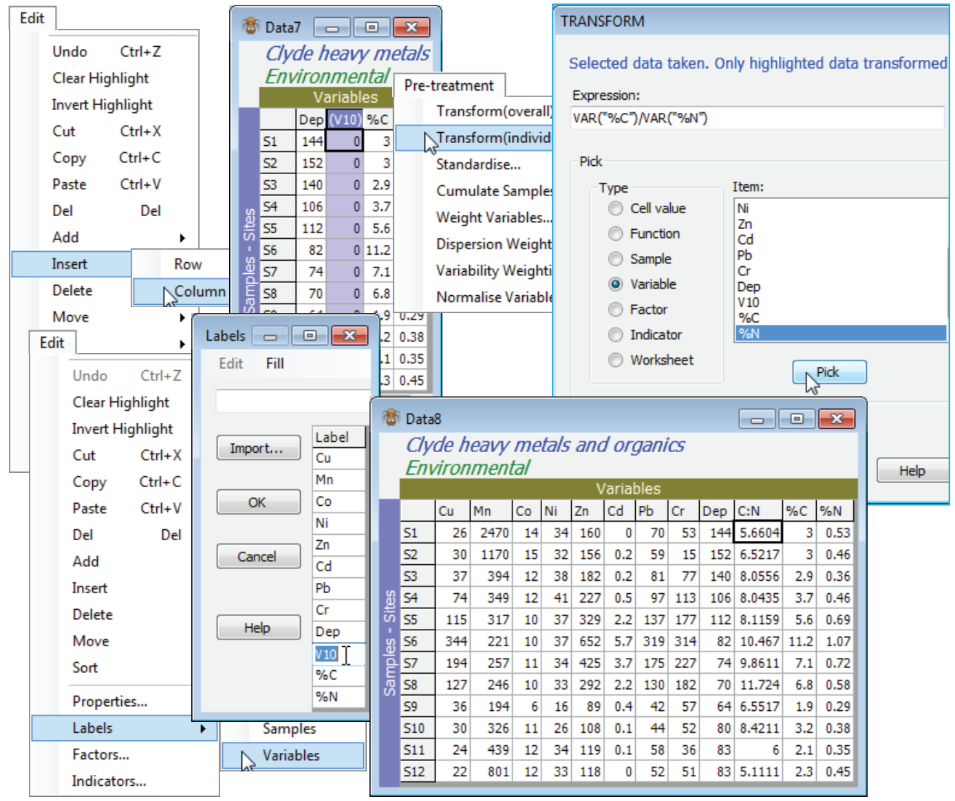
For an example of an Expression combining two (or more) variables, use the Clyde environmental sheet but copy it (Tools>Duplicate), which is always a good idea when experimenting! The aim is to create a new variable (column) which is the C:N ratio, so first Edit>Insert>Column, which will be placed to the left of the current cursor position – here this might logically be on the %C column. [Incidentally, remember that the new Edit>Undo will step back any Edit operations like this which change the current data matrix, rather than creating a new sheet (where a new sheet is created it can always be deleted if incorrect, and the process repeated). And note that Edit>Undo is local to the currently active matrix, so will undo the last such operation on this sheet, irrespective of whether similar operations have been performed since, on other sheets in the workspace – they will not be wound back by Edit>Undo if their sheet is not the active one]. The new column is labelled (V10) because of its position in the matrix, and the calculation we do to create the C:N ratio is to be put in this column, so it needs to be highlighted. Take Pre-treatment>Transform(individual) and delete the V from the Expression box (that refers only to values in the new column, which we shall not be using – they are all zero of course). Then, under Pick, take (Type•Variable) & (Item: %C)>Pick) and follow by (Type•Variable) & (Item: %N)>Pick), which creates the two variables we need in the Expression box. Manually insert the divide symbol (/) between them, to give the (Expression: VAR(“%C”)/VAR(“%N”)), and OK now gives a new sheet with the added C:N ratio variable V10. (Even if you chose to tick the (✓Rename variables) box, the new name will still be clumsy and it would be better to change it to C:N using Edit>Labels>Variables).
An alternative, e.g. if you just intend to take this new variable back into the earlier transformed sheet, is not to insert a new blank column, instead just highlighting the %C column (which will now be V in the Expression box), and Pre-treatment>Transform(individual) with (Expression: V/VAR(“%N”)). In the new sheet, this will have overwritten the %C row with the C:N ratio. Either way, you can now put the new C:N variable back into the transformed sheet simply by highlighting it, then Select>Highlighted and Tools>Merge it with the transformed sheet, taking the defaults.
Expressions combining worksheets
Similarly, expressions can combine samples, or even factors (or indicators) on those samples (or variables) – and expressions can even incorporate different worksheets. In fact some of the most useful applications of complex expressions are in combinations of data from related worksheets, such as the abundance and biomass arrays of macrofaunal assemblages from the Clyde study. The key facts to keep in mind when constructing complex expressions are that V stands for any entry in the active sheet that is highlighted, that the result will be placed only into these highlighted cells (which could mean the whole array, if there is no highlighting), and that maintaining strict labelling across worksheets will make it easier to understand what the expression calculates for each cell. (Though, as elsewhere in PRIMER, if Transform(individual) is given two data sheets that have conformable dimensions but not consistent labelling, then it will give the user the chance to relax strict matching and assume that samples or variables are presented in the same order).
If not already in the workspace, open Clyde macrofauna counts and Clyde macrofauna biomass. One useful way of combining abundance and biomass information from the same set of samples is in equation (15.1) of CiMC, namely an allometric equation for pseudo-production, $P = A^{0.27} B^{0.73}$. With the abundance sheet active, turn off any highlighting with Edit>Clear Highlight, or higlight everything (the effect is the same), then take Pre-treatment>Transform (individual)>Expression: (V^0.27)*(Work(“Clyde macrofauna biomass”)^0.73). You can use (Type•Work¬sheet) & (Item: Clyde macrofauna biomass)>Pick to give you the syntax for the second sheet but type the rest; the counts of the first sheet are held in V ($\equiv$ Work(“Clyde macrofauna counts”)), since that is active. You should definitely uncheck (✓Rename variables) so that the species names remain intact.
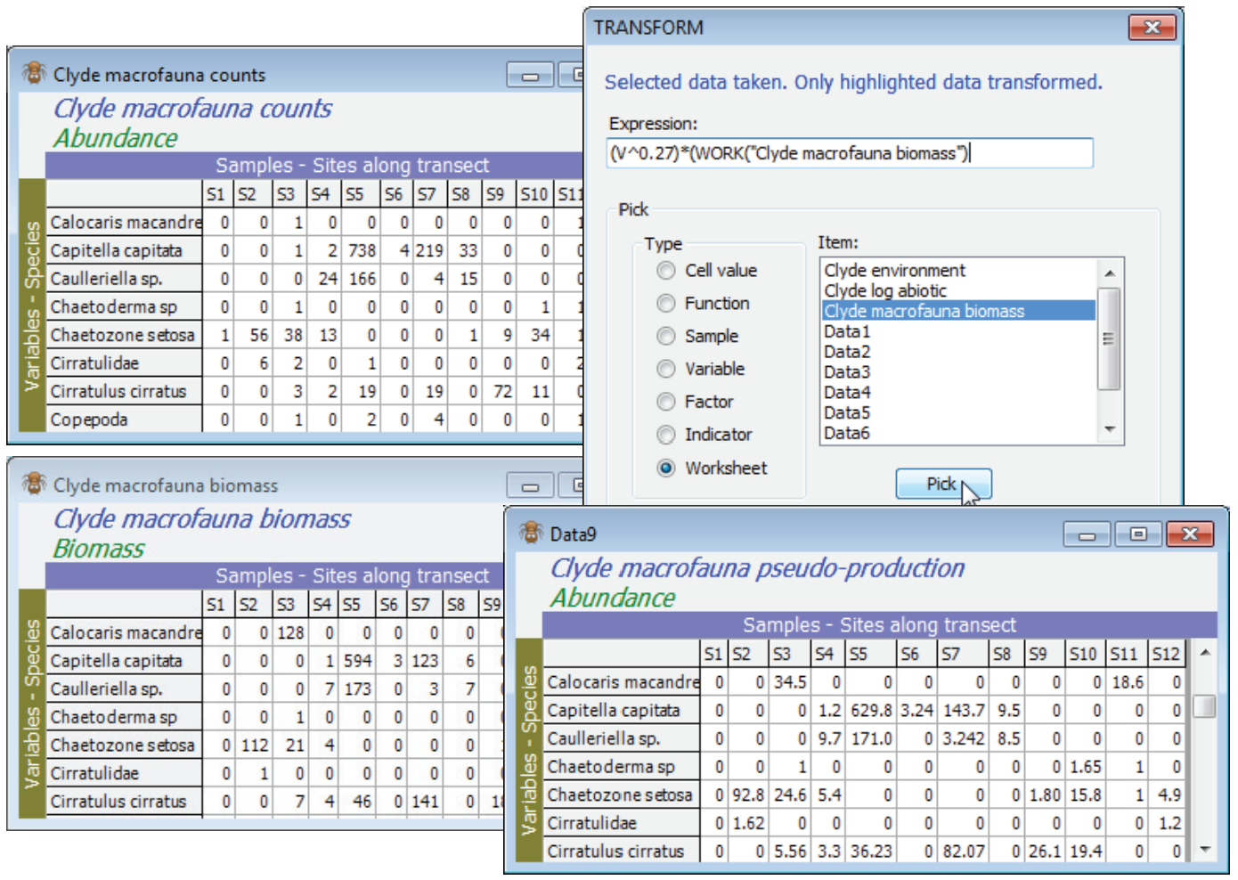
Average body mass matrix (B/A)
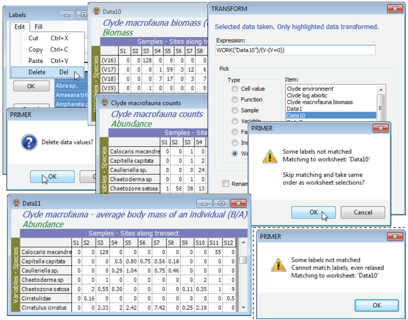
A useful variation of this, but one which needs more care, is to compute average body mass of each species in each sample. This is simply B/A, but needs to cater for the many cases when A (and B) are zero and a simple ratio is undefined. With active sheet Clyde macrofauna counts, so that V is again the counts, Pre-treatment>Transform(individual)>Expression: Work(“Clyde macrofauna biomass”)/(V – (V=0)) will do the trick, because when V>0 the expression (V=0) gives the value 0 (false), so that the correct ratio of B/A is calculated. However, when V=0 the expression (V=0) returns the value -1 (true). The bottom line is then 1 and the result of the ratio is a reasonable value of 0. This assumes that B=0 when A=0 of course! [This, incidentally, is something that can be checked by running Abundance-Biomass Comparison curves, described in Section 16, since the Analyse>Dominance Plot (ABC) routine explicitly checks for incorrect matrix entries which have A=0 but B>0; the converse is perfectly permissible – the weight of all organisms of a species in a sample might be too small to register – but this does not cause a problem with a B/A calculation).]
An illustration of error trapping and relaxation of strict matching, in Pre-treatment>Transform (individual) with matching of entries, is obtained by copying Clyde macrofauna biomass with Tools>Duplicate, then Edit>Labels>Variables on this to delete all the species labels (click the Label header and hit the delete key or Edit>Delete). A sheet cannot function without labels so PRIMER substitutes its own defaults of (V1), (V2), etc. Now run the above calculation on Clyde macrofauna counts, but with the relabelled biomass sheet (Data10 below) replacing the original biomass sheet. A warning message says that it could not find (variable) labels to match, but the two matrices are the same size so the option is given of proceeding anyway, on the assumption that the species order matches. We know it does here, so continue, to give the desired B/A matrix, and the original species labels will be present in the resulting new sheet because these are always taken from the active matrix, in a case such as this. Re-run having deselected one of the rows in Data10, however, and an irrecoverable error message occurs – a match is impossible because the variable labels do not match and neither does the number of variables in the A and B matrices.
Transform on resemblances; Combining resemblances
Transforming resemblances remains in the Tools menu in PRIMER 7, since it is not an option for pre-treatment of data matrices prior to resemblance calculation (which characterises the other items on the Pre-treatment menu). Although not commonly required, it facilitates at least a couple of interesting analysis concepts. One is really outside the scope of this manual, namely to examine the extent to which the semi-parametric PERMANOVA tests are robust to (monotonic) transformation of the resemblance values, transformations which would not change the ANOSIM test results in any way (since they are based only on the ranks of the resemblances). It is empirically well-known, for example, that the square root of Bray-Curtis (unlike Bray-Curtis itself) does not give negative eigenvalues for the high-d PCO ordination which underpins the approaches in PERMANOVA+. Whether the consequentially poorer low-d PCO representation is a price worth paying for a PCO space without imaginary axes must be open to question, however. Tools>Transform on a single resemblance matrix provides a basic tool to assist in following up such questions. More simply, we have already seen it used (under Correlation as similarity in Section 5) to turn a correlation with values in ( 1, 1) into a similarity over (0, 100) by use of the transform Expression: 100*Abs(V).
Another use of Tools>Transform on resemblance matrices is also less esoteric and potentially of substantial practical benefit. It provides an interesting solution to the handling of ecological data matrices from mixed faunal types, e.g. counts of motile organisms and cover of colonial species within the same rocky-shore quadrats. This type of problem was raised earlier (end of Section 8), when two resemblance matrices over the same set of samples were combined in a single MDS, by minimising an average stress function. The difficulty with that approach is that it only generates an MDS, and many of the methods in PRIMER do not work in the approximate low-d space of an ordination but on the full resemblance matrix (or usually its ranks). However, whilst counts and area covers are difficult to scale in relation to each other in a single data matrix, it is not difficult to calculate Bray-Curtis similarities (say) for a count matrix and a cover matrix separately, for the same set of samples, and then simply average the two resemblance matrices over every matching pair of entries using Tools>Transform, using a similar worksheet-based transform expression to that previously demonstrated. (Dis)similarity values in the range (0, 100) for both matrices will stay in (0, 100) under the arithmetic averaging expression of (A+B)/2 (or a weighted form, (3*A+B)/4, if the contribution of counts is considered roughly three times as important as that from area cover). Geometric averaging of the type seen above is also possible, e.g. (A*B)^0.5 or (A^0.75)*(B^0.25). If the two resemblance matrices are not on a common scale and direct averaging is not appropriate, a simple solution would be to run both through Tools>Rank distance, putting them on a common scale – and fitting well with PRIMER’s non-parametric approach – then averaging as above and re-ranking (though the latter is unnecessary for most PRIMER routines, which do their own ranking).
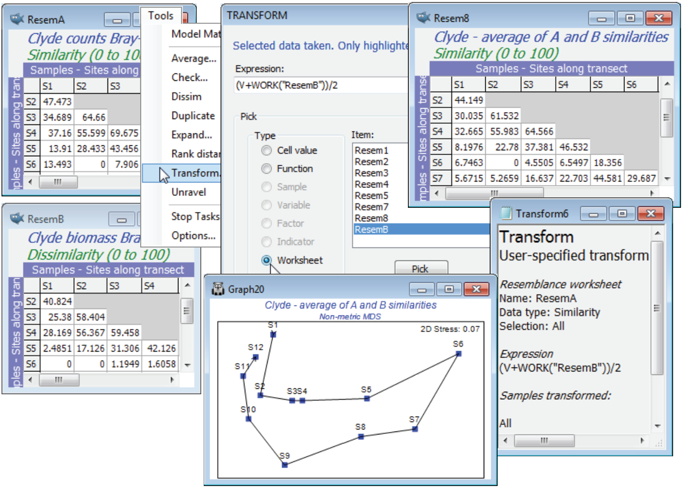
A simple example using two resemblance matrices can be constructed with the Clyde data, namely the Bray-Curtis site similarities averaged over abundance and biomass measures. So, instead of combining the data matrices (as in the earlier $A^{0.25} B^{0.75}$), we average the A and B resemblances. There is likely already to be a Bray-Curtis similarity matrix based on the square-root transformed biomass data from Clyde macrofauna biomass in the workspace (rename it ResemB) and you should now also compute Bray-Curtis similarities from Clyde macrofauna counts, this time on fourth-root transformed data (there is no reason why a different transform should not be appropriate for abundance than for biomass data). Then with the abundance similarities ResemA as the active sheet, take Tools>Transform>(Expression: (V+Work(“ResemB”))/2), change the title of the result appropriately, and run Analyse>MDS to compare this with the earlier (ranked) biomass MDS.
Tools menu - other items; Tools Options menu
Tools operations on resemblances which are discussed elsewhere are: a) Dissim and Unravel in Sections 5 & 6 – the former turns similarity into dissimilarity, or vice-versa, and the latter creates a single column of entries from unravelling rows of the triangular matrix; b) Model Matrix and Expand in Section 14 – these are less trivial and need contextual explanation; and c) Stop Tasks in Section 6 (self-explanatory). That leaves only Tools>Options, PRIMER’s default settings.
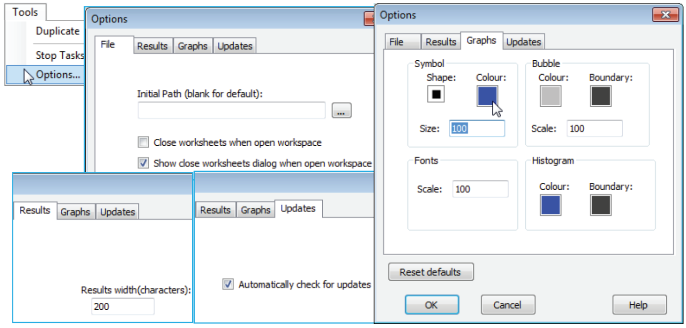
Options appears on the Tools menu whatever the type of active window. The items on the File tab were seen in Section 1, namely the default setting for the initial directory on launch of PRIMER from the Windows desktop (in general there is not a strong incentive to change this from its default blank entry since, once closed, PRIMER will relaunch to the last used directory), and whether, on opening workspaces, they are displayed with full branches unfurled or not (this can take some time for very large workspaces). There is also the option to suppress the initial dialog about this feature, which is otherwise displayed every time a workspace is opened. When on this, or any of the other tabs, the factory default settings for PRIMER (for all tabs) can be re-instated by Reset defaults, and those defaults are as illustrated in the dialog boxes below.
The Results tab contains a single, little-used item, which just determines the page width for results – the number of characters in the fixed-spaced font used for Results windows. This is initially set to 200 and only comes into play with the few routines (SIMPER and DIVERSE, Sections 10 and 15) which can generate wide lists of results. If this default is set to a smaller value than will allow a single span of results columns, they are split and listed a batch at a time. In practice, the DIVERSE routine essentially produces a matrix of samples (rows) by diversity indices (columns), so it will usually be preferable to direct this to a new worksheet, where it can be further plotted or analysed as a multivariate array (or be exported to Excel or a univariate statistics package). The Updates tab similarly concerns a single issue, this time a check box (new to PRIMER 7) to specify whether the software should automatically check the PRIMER-e server for existence of a maintenance update, and if it finds one, to ask the user whether they wish to download this at that point in time or not.
The Graphs tab is the most likely to be used on a regular basis, since this sets some of the global defaults for all plots. In the Symbol area, Shape, Colour and Size can be set for all graphs on which a single symbol type is plotted, e.g. a draftsman plot, Shepard diagram, an ordination graph which does not plot different symbol types by factor or, indeed, a bubble plot for a single variable with no factor used (with a factor, or for >1 variable, the bubble colours are determined by the appropriate Key dialog). The Bubble area therefore only controls the inner and boundary colours for the bubble key when it accompanies a bubble plot utilising more than one different coloured bubble, hence the default of a neutral grey with black boundary to avoid a misleading colour synchrony with any of the factor levels. The Bubble Scale box does, however, apply to all bubbles because it sets the size for a bubble at the maximum variable value given by the Bubble key. In fact, it provides the default for the (Bubble scale:) box in the Graph>Special>Main>Bubble area, and the Symbol Size default similarly sets the value in the Symbol area of the Graph>Sample Labels & Symbols tab (hence applies also to symbol sizes when plotted by factor levels). The Fonts Scale box likewise fixes the displayed default for (Overall font scale:) on the Graph>General tab, so applies to all fonts. Lastly this Graphs tab sets the default Histogram inner and boundary colours. It must be appreciated that default changes are not retrospective; they apply only to plots created after any default changes.