13. Linking assemblage to environment (BEST: Bio-Env, LINKTREE)
- BEST rationale
- Bio-Env vs BVStep
- Change to active sheet for BEST
- Grouping variables in BEST
- Selecting variables & resemblance
- 2-way BEST
- The BEST matching statistic, $\rho$
- Limiting the number of combinations
- BEST results detail
- (Messolongi diatoms & abiotic data)
- Global BEST test
- Linkage trees – rationale
- Non-metric, non-linear, non-additive
- LINKTREE (Messolongi lagoons data
- SIMPROF test in LINKTREE
- Missing data in linkage trees
BEST rationale
The main rationale for the Analyse>BEST procedure in PRIMER is to find the best match between the multivariate among-sample patterns of an assemblage and that from environmental variables associated with those samples. The extent to which these two patterns match reflects the degree to which the chosen environmental data ‘explains’ the biotic pattern. This leads naturally to the idea of searching over subsets of the abiotic variables for a combination which optimises that match, namely the best explanatory variables – see Chapter 11 of CiMC for details of the method¬. The concept is a more general one (see also Chapter 14), and BEST can equally be used to find: subsets of taxa which best match a fixed environmental data set (e.g. vulnerable and opportunist species characterising a known impact gradient); subsets of biota which best match a different biotic matrix (e.g. key coral species which may be structuring a reef fish community) or even the same biotic matrix (e.g. a small subset of species, perhaps chosen from a set of easily-identified taxa, which generates the same multivariate sample pattern as would the full assemblage). Parallel applications for different data types can also be envisaged, for example: a subset of tissue contaminant levels that best ‘explain’ a suite of biomarkers, or conversely, a subset of biomarkers that best identify a body burden contaminant gradient; a subset of geomorphological variables that best characterises an existing classification of rivers or coasts; a small set of morphometric or genetic/molecular measures that is as effective as a larger set in discriminating two putative species, and so on.
Bio-Env vs BVStep
BEST amalgamated the earlier (PRIMER 5) BIOENV and BVSTEP procedures (hence BEST = Bio-Env + Stepwise) since they had an identical purpose – to search for high matrix correlations, rank-based, between a fixed sample similarity matrix (typically from a species assemblage) and resemblance matrices generated from different variable subsets of a supplied data matrix (usually a transformed and normalised suite of environmental variables presumed to include those ‘driving’ the assemblage structure). The only difference in operation is that BIOENV carries out a complete search of all possible combin¬ations of variables from the datasheet, whereas BVSTEP caters for the common situation in which there are too many variables to do an exhaustive search, and a forward-stepping and backward-eliminating stepwise procedure is necessary to arrive at a (possibly) optimal set. Within Analyse>BEST, the first choice is therefore of Method•BIOENV or Method•BVSTEP. (BVSTEP will be discussed in Section 14, where it becomes essential for use on biotic matrices).
Change to active sheet for BEST
In what is one of the very few examples of ‘moving the furniture around’ between PRIMER 7 and earlier versions, the active window for a run of Analyse>BEST is no longer the data matrix of (usually abiotic) variables, from which selections are made to best match to a fixed resemblance matrix (usually of assemblage pattern), but the converse, i.e. Analyse>BEST is run from an active sheet which is the fixed resemblance matrix, and a secondary matrix supplied which is the (abiotic) data matrix from which variables are selected. There are several good reasons for this switch, the most compelling of which is that it allows much greater consistency in the way PRIMER decides which samples to use in an analysis when there is only a partial match of sample labels between the two data sets. The consistent rule now, throughout PRIMER (and PERMANOVA+), is that the active matrix (in its currently selected form, if any selections are in place) determines that sample set. Any secondary matrix supplied to the routine (here, the abiotic variables) are treated as a ‘look-up’ table from which the required set of samples is extracted. Thus, the environmental matrix can (and sometimes will) cover a much wider range of sites than are utilised in the current community samples – they might for example be interpolations from some physico-chemical or remote-sensing model for the whole region. What is required is that BEST can find all (biotic) resemblance sample labels in the (abiotic) data matrix, otherwise an error is returned – with the usual relaxation of strict label matching that if the two matrices have exactly the same number of samples, i.e. BEST will ask the user if it should should proceed on the assumption that the samples are in the same order. [Other benefits from switching the active matrix for BEST include consistency with the DISTLM routine in PERMANOVA+, which is the semi-parametric equivalent to the non-parametric BEST program, and a close multivariate analogue of (univariate) multiple linear regression. In standard statistical thinking, the response here is the community sample, thought of as subject to sampling/ spatio-temporal variability and that is regressed on the observed values of the explanatory variables (the latter considered fixed, under a conditionality argument). PERMANOVA+ routines thus start from the response, as given by the community resemblances – which are always the active sheet – and explanatory variables (in DISTLM), covariates (in PERMANOVA) etc are always secondary.]
Grouping variables in BEST
After the initial choice of Method, the next area on the BEST dialog inputs the explanatory (fitted) data worksheet and, in a new option in PRIMER 7, allows the user to specify an indicator for that sheet which groups its variables into indivisible sets. For example, one ‘explanation’ of differences in community structure might simply be geographical location. If that is a latitudinal gradient it could be represented by a single explanatory variable, but if the samples have 2-d rectangular co-ordinates (or even 3-d), then it would not make sense for the BEST search procedure to consider explanations which included the x but not the y co-ordinate. If this pair of variables are specified as a group – they have the same level of the indicator – then they will be selected (or not) as a single unit. (Whether it is sensible to include geographic location in the explanatory set for a community pattern is another matter altogether, since location cannot be causal per se – an organism does not know its GPS co-ordinates! Instead, the model is more likely to be that of species responding to other enviromental variables which are changing with geographical position, and those should be the variables in the explanatory set). Other examples of grouping might be to separate variables of different types: Valesini FJ et al 2014, Estuar Coasts 37: 525-547 give a BEST analysis of this sort in which estuarine fish communities are related to groups of variables representing wave exposure, substrate type, marine water intrusion etc, in order to determine if one or more sets of variables are particularly influential – Chapter 11 of CiMC gives slightly more detail.
Selecting variables & resemblance
After the (✓Group variables(indicator)) check box, the next option is a Select variables/groups button, which gives the usual type of selection dialog with three panes. The default is for all the variables – for which read ‘groups of variables’ if the previous check box is ticked – present in the (Fitted data worksheet:) to be displayed in the (Available:) pane. These will then be picked and dropped in all combinations. Variables that are moved to the (Force exclusion:) pane will never enter any of the combinations considered, e.g. you might choose to exclude a variable which is very highly correlated with another in the list. Those variables in the (Force inclusion:) pane will be included in every combination, e.g. you might know that a particular environmental variable is causal for the assemblage, and therefore always want to include it when considering whether adding other variables improves the ‘explanation’. The choice of (Resemblance:) coefficient for the explanatory variables then follows. The default for this is determined by the datasheet type – often environmental, and thus Euclidean distance – but can be altered to any of the numerous measures which PRIMER offers, through the Change button. Importantly, for environmental variables on different scales, the supplied explanatory variables worksheet should be in its normalised form before Analyse>BEST is run – there is no option within the dialog box to add this pre-treatment step before selection of Euclidean (or other) distance measure.
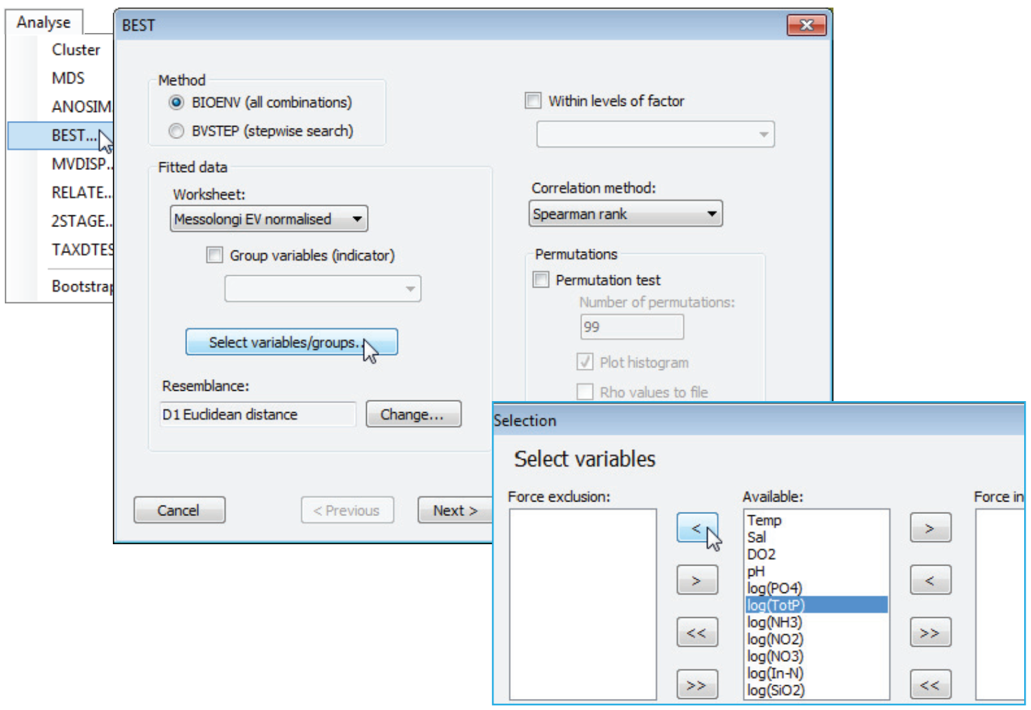
2-way BEST
On the right of this main dialog box for BEST is another option new to PRIMER 7, also covered in Chapter 11 of CiMC, namely the check box (✓Within levels of factor ). Essentially, this gives a constrained (or 2-way) BEST procedure in which the match in sample patterns between (usually) abiotic variables and the assemblages is calculated separately for each level of the supplied factor, and the appropriate matching statistic (a matrix correlation) averaged over those levels. Selection of the variables is made simultaneously in all levels of that factor, and the optimum match is therefore given by the variable set which succeeds in maximising this averaged matrix correlation. The idea is that there may often be situations in which the dominant differences between communities are due to an (unordered) categorical factor, which cannot be simply accommodated by adding another (ordered) variable to the abiotic matrix, and is perhaps a nuisance factor in trying to understand the detailed relationship between abiotic and biotic patterns – its effect is fully removed by matching only within the strata of this factor. The analogy with 2-way ANOSIM is strong, e.g. removing the effect of Site when testing for differences over Time, by constructing an R statistic for a Time test separately for each Site, and averaging them. So this analogous matching procedure can be thought of as a 2-way form of BEST. Just as with ANOSIM, it may be possible (and sensible) to run BEST entirely separately within each stratum of the nuisance factor, e.g. match abiotic to biotic patterns completely independently for each of a small number of geographical regions. However, where there are rather few samples in each region, 2-way BEST provides a ‘half-way house’ in which matching is carried out separately for each region but with common choice of the abiotic variable set, which makes sense if there is not a strong interaction between the effect of an environ¬mental variable and the region (e.g. an interaction would be when salinity is crucial to the community in region A but, though varying equally greatly in region B, has no effect on the community structure there). Under these (additive, not interactive) conditions, such a constrained, 2-way BEST routine may lead to a much more incisive (powerful) analysis.
The BEST matching statistic, $\rho$
On the mid-right of the main dialog for BEST, the box headed (Correlation method:) now offers three non-parametric choices and one parametric correlation: Spearman rank, Weighted Spearman rank, Kendall tau and Pearson, covered in equations (11.3), (11.4) and (2.3) respectively in CiMC. These are the measures of agreement (matching statistics) between the two resemblance matrices, e.g. biotic and abiotic, and correlations ($\rho$) are calculated by matching element to element. The logic is that if the true driving abiotic variables are selected, and two sites have very similar suites of values for these, then the assemblages will also be very similar (and vice-versa), so the triangular matrix elements should rank in the same order. Ranks are usually appropriate not only because of their central role in PRIMER, underlying a non-metric MDS ordination and the hypothesis testing procedures in ANOSIM and RELATE, but also because the two resemblance matrices may use entirely different coefficient types, e.g. Euclidean distance in (0, $\infty$) and Bray-Curtis in (0,100). Whilst the above logic then leads one to expect a monotonic relation between their values, there is no reason to expect a linear relationship between a distance and a finite-range dissimilarity, so standard Pearson correlation will generally be less effective. However it is included in PRIMER 7 to cover situations in which, for example, two sets of Euclidean distances, or two sets of Bray-Curtis dissimilarities are being matched, and a standard correlation may then be more acceptable. Though weighted Spearman was constructed to be more relevant to this specialised case of matrix correlations (rather than standard rank correlations of two variables with independent entries), in practice there is rather little to choose between the three rank-based coefficients.
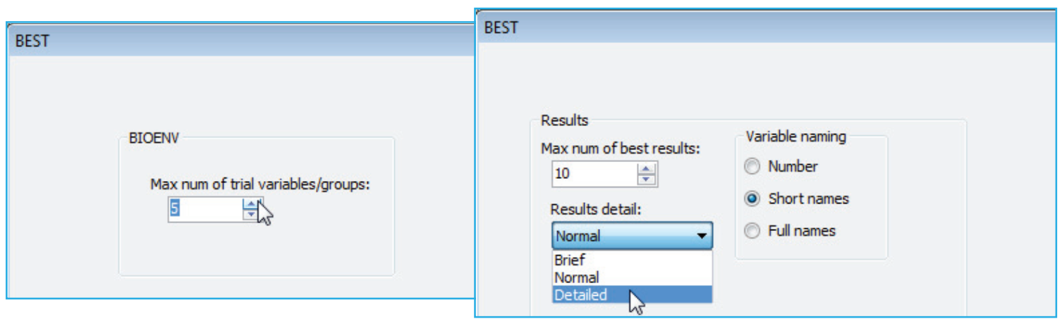
Limiting the number of combinations
The final area of the main BEST dialog, headed Permutations, which carries out the global BEST test for statistical significance of the best matching combination of variables, is deferred until later in this section. The Next > button, under (Method•BIOENV), gives a dialog with a single entry, a choice of (Max num of trial variables/groups: ), for which 5 is the default. This limits the search to $\le$5 (abiotic) variables at a time, and this maximum number should be increased, where feasible. A default of the total number of input variables is not used because the number of combinations of these in an exhaustive search could be very large: for p variables there are c = 2$^p$ – 1 combinations, and a practically realistic limit therefore has to be about p = 17 (giving c $\approx$ 100,000). The context for Section 13 is the matching of subsets of environmental variables to assemblage patterns. Quite often, the number of abiotic variables is then <17 or, if not, the number should probably be pruned before running BEST – so only a full search (BIOENV) will be illustrated now. BVSTEP could be run in much the same way on a larger set, but the reason this is likely to prove unattractive is that, with so many abiotic variables, it is inevitable that they will be strongly inter-correlated. There are then a plethora of equally good solutions and a rather unfocussed interpretation. Deletion of all but one of a highly mutually-correlated set of variables and/or prior reduction to one representative of each different type of environmental variable, may be desirable, just as in multiple linear regression (see the discussion in Chapter 11 of CiMC). In some of the other applications – e.g. when the data matrix is of species variables and a priori selection defeats the point of the analysis – the stepwise form (Method•BVSTEP) will be essential, and such an example is seen in Section 14.
BEST results detail
Previous versions of PRIMER used only the variable number in these tables, with a list at the start of the results relating those numbers to the variable labels. This made the large tables cumbersome to interpret, so PRIMER 7 offers three options: variable naming by (•Number), (•Short names) or (•Full names). The last of these is the full variable label and the middle option a truncated form, each variable with as few of its initial characters as are sufficient to make the names distinct. This much improves the readability of the output, but there are occasions when it is still desirable to re-run BEST with numbers, so that the best set can be easily selected from the original matrix with Select>Variables>(•Variable numbers: ), copying and pasting the number string to this box.
(Messolongi diatoms & abiotic data)
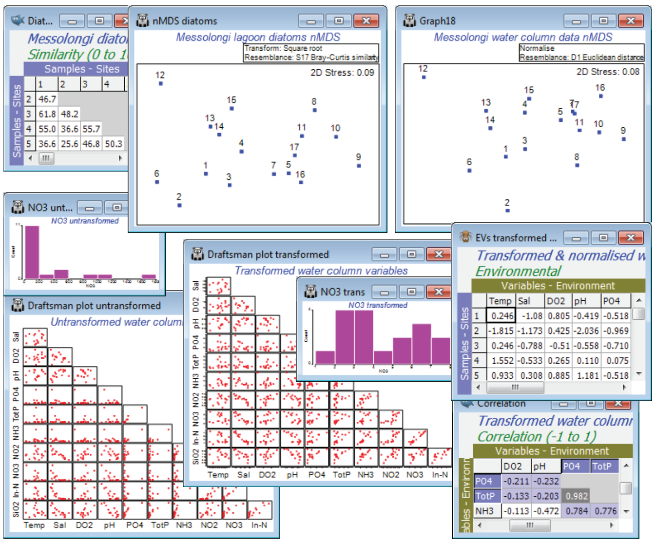
A study of diatom assemblages (abundances of 193 species) at 17 sites in the lagoons of Messol-ongi, Aitoliko and Kleissova in Eastern Central Greece was undertaken by Danielidis DB (1991), Ph.D. thesis, Univ Athens. At each site, a suite of 11 water-column data was also recorded: Temperature, Salinity, DO$_2$, pH, PO$_4$, Total P, NH$_3$, NO$_2$, NO$_3$, Inorganic N and SiO$_2$. The data files are Messolongi diatom density and Messolongi environment in C:\Examples v7\Messolongi diatoms. This is an ecological study of how the diatom communities relate to the water-column variables.
Square-root transform the abundance file and take Bray-Curtis resemblances, plotting the nMDS as usual. Plots>Draftsman Plot or Histogram Plot show that a log transform would be desirable on the nutrient concentration variables PO$_4$, TotP, NH$_3$, NO$_2$, NO$_3$, In-N and SiO$_2$, but Temp, Sal, DO$_2$ or pH do not need any transformation. As in the previous section, carry this out by highlighting (not selecting) the variables to be transformed and take Pre-treatment>Transform(individual)>(Expression: log(V)), unchecking the (✓Rename variables) box – readability of the BEST output is improved if not all the variable names look like log(...)!, so bear in mind that PO$_4$ means log(PO$_4$) etc, from now on. Re-running Draftsman and Histogram Plots, and also taking (✓Correlations to worksheet) for the former, shows that the distributions now have greatly reduced right-skewness. Two variables, PO$_4$ and TotP are seen to be strongly collinear, and it will make sense to drop one of them in the BEST run – they are, in effect, the same variable. You can pick out which are the very strongly correlated variables by Select>Samples>(•Values>0.95) on the correlation matrix produced by the draftsman plot – and potentially repeat again with (•Values<-0.95), though there are none of the latter here. This will display only those rows and columns of the triangular matrix with a value >0.95 somewhere, just PO4 and TotP in this case. On the transformed data, take Pre-treatment>Normalise variables, and the among-sample relationships, in terms of these 10 abiotic variables, can then be seen either by Analyse>PCA directly on this matrix or calculating Euclidean distance and putting that into MDS. As expected, since both are based on Euclidean distance, the two ordination methods for the abiotic data give very similar 2-d plots but more remarkable is the near-perfect match of biotic and abiotic analyses – the 193-species diatom community is highly predictable from knowledge of these 10 water-column variables.
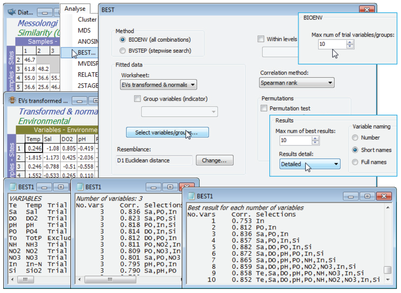
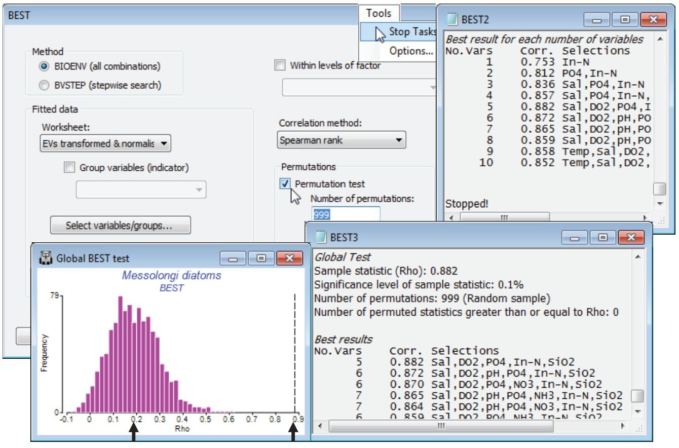
In fact, the match is even better with fewer abiotic variables. With the diatom resemblance matrix as the active sheet, run Analyse>BEST>(Method•BIOENV) & (Worksheet: EVs transformed & normalised), forcing exclusion of TotP under the Select variables/groups button, with the default of Euclidean resemblance and (Corr¬elation method•Spearman rank), and leaving the Permutation box un¬checked. On the Next > dialog, increase to (Max num of trial variables/groups: 10), since all 1023 combinations will run in a reasonable time. On the final dialog, (Results detail: Detailed) and (Variable naming•Short names). The results window and particularly the summary table of Best results for each number of variables shows that $\rho$ is maximised (at 0.88), for the 5 variables: Sal, DO$_2$, PO$_4$, In-N, SiO$_2$ and slowly decreases beyond that, as more variables are added. The best 3-variable solution (Sal, PO$_4$, In-N) does nearly as well ($\rho$ = 0.84), and on the principle of parsimony might be preferred as a simple ‘explanatory’ set of abiotic variables for these diatom communities. Causality, of course, is not established – see the comments in Chapters 11 and 12 in CiMC.
Global BEST test
The question of statistical significance testing on the results of the Bio-Env (or BVStep) procedure naturally arises. Section 14 describes Analyse>RELATE, a (non-parametric) form of Mantel test. For any two independently-derived resemblance matrices, defining the relationships among the same set of sample labels, one can use permutations to test the null hypothesis H$_0$: no agreement in multivariate pattern. The measure of agreement is the (usually rank) correlation coefficient $\rho$, discussed above, between the corresponding elements of the two triangular arrays, with $\rho$ = 0 representing the null hypothesis. The $\rho$ values that it is possible to observe by chance, if the null hypothesis is really true, can be generated by randomly permuting one set of sample labels relative to the other (thus destroying any real link) and recalculating $\rho$, over many random permutations. RELATE could therefore be applied to testing agreement between an assemblage and the full set of environmental variables for the same sites (though not for all other linkage problems mentioned earlier, e.g. between the full assemblage and a subset of conspicuous species, since independence is violated – any subset of species will bear some relation to the full set). It is important to realise, however, that RELATE cannot be applied to the subset of environmental variables that result from a run of BIOENV: these have been selected precisely to maximise the matching coefficient $\rho$ with the assemblages. Even where there is no real match, the optimum $\rho$ produced by BIOENV will inevitably be >0. We need a test which allows for this selection bias, and this is the global BEST test (Clarke KR et al 2008, J Exp Mar Biol Ecol 366: 56-69, and Chapter 11, CiMC), a permutation procedure accessed on the first dialog box from Analyse>BEST. The idea is simple: randomly permute one set of sample labels in relation to the other, then run through the full BIOENV (or BVSTEP) process to generate the best match $\rho$. Another permutation of the labels is then generated and the BIOENV run repeated again, and so on (for 99 times by default, because of the intensive computation involved – but preferably more). This produces 99 values of $\rho$ in a histogram, which represents the null hypothesis. The real $\rho$ is compared with these, as for any PRIMER permutation test – if it is larger than any of them, then the null hypothesis can be rejected at p<1% significance. Actually, this is the sole example in PRIMER of a statistic ($\rho$) which does not take the value 0 for the null hypothesis – as indicated above, the mean $\rho$ is certain to be >0 under H$_0$.
When the new 2-way BEST routine is run, by taking the option (described earlier) to remove the effect of a categorical variable by matching only within its levels, the test proceeds in the same way but with a constrained permutation of biotic sample labels within – not across – those levels.
From an active sheet of the lagoon diatom resemblance matrix, re-run Analyse>BEST>(Method• BIOENV) & (Worksheet: EVs transformed & normalised) with most options as before but this time taking (Permutations✓Permutation test)>(Number of permutations: 999) & (✓Plot histogram), and (Variable naming•Full names). On a slow machine, or with more samples than here, you will probably need to reduce the number of permutations to 499, or 199, or 99. The latter is adequate if the result is clear cut, but results in a much less smoothed histogram, and you will wish to calculate more in border¬line cases. Remember that you can use always use Tools>Stop Tasks (or the icon on the Tool Bar  ) to interrupt a permutation test that, from observing the green progress bar, is clearly going to take too long – note that since it computes and outputs the BEST results tables for the real data before embarking on the random permutations, you will not lose these if you stop the routine prematurely. An alternative is to multi-task, carrying on with other PRIMER activities as the permutation test runs in the background – this is not a problem. In addition to generating a null distribution histogram (for which you can change the bin size, colours etc with Graph>Special as usual), the test adds a small section to the results window, headed Global Test, whose format is as for the ANOSIM test, Section 9. It gives the real value of $\rho$ and its % significance, 100$\times$(1+(no. of permuted $\rho \ge$ observed $\rho$))/(1+no. of perms). The real $\rho$ (0.88) is well to the right of the upper tail of the null distribution, p<0.1% (i.e. P<0.001). Note also that the mean of the histogram is not zero but around $\rho$ = 0.2. The strong selection pressure, over a large number of variable combinations, is able to produce an artefactual match up to about $\rho$ = 0.4 or even 0.5, though there is no question that the null hypothesis is rejected here – such a good match of water column indices to the diatom assemblages, as seen in the earlier biotic and abiotic MDS plots, clearly cannot be due to chance. A final step would be to select only the BEST set of abiotic variables and repeat the Euclidean MDS.
Linkage trees – rationale
Another technique for linking sample patterns based on assemblage data to a suite of environmental (or other) explanatory variables was also discussed in Clarke KR et al 2008 J Exp Mar Biol Ecol 366: 56-69 (see the last topic in Chapter 11, CiMC). The well-established statistical procedure of Classification And Regression Trees (CART) was further developed in an ecological context by De’ath G 2002, Ecology 83: 1105-1117, termed Multivariate Regression Trees (MRT). PRIMER implements a modification of this, in a form which is consistent with the non-metric philosophy underlying the rest of the package. The connection with regression is minimal (and confusing) so the more descriptive term linkage trees is used by PRIMER for its variation of the procedure. Its real affinity is with Cluster analysis (Section 6, under heading Binary divisive clustering), and it is therefore accessed in PRIMER v7 by running Analyse>Cluster>LINKTREE. In fact, it is a form of constrained binary divisive clustering in which the successive divisions of the full set of biotic samples, seen in the unconstrained divisive clustering of Analyse>Cluster>UNCTREE (Section 6), are limited to those splits of each group (into two new sub-groups) which have an explanation in terms of larger or smaller values of a specific explanatory (typically abiotic) variable – consistently so on either side of that divide. In other words, all constraints are a threshold inequality on a single abiotic variable and this set of inequalities form the possible ‘explanation’ for the biotic structure.
We have already seen two techniques for linking assemblage patterns to abiotic variables: bubble plots (Section 8) and the above BEST procedure. BEST has the advantage of looking at the abiotic variables in combination, trying to identify a subset which is sufficient to ‘explain’ all the biotic structure capable of explanation, and the matching procedure takes place in the full high-d space, i.e. on the respective resemblance matrices. But on its own, this falls short of a full interpretation because it does not demonstrate which variables take high or low values for which samples. Bubble plots give the latter but are only satisfactory where the low-d biotic nMDS has acceptable stress as an approximation to the full biotic pattern. Linkage trees can fill this gap: they can take the subset of abiotic variables identified by BEST, and use them to describe how the assemblage samples are optimally split into groups (in the high-d space), and interpret this, e.g. Group 1 communities have Salinity<23ppt but Group 2 are from >26ppt (with no samples between these salinity thresholds). Group 1 and 2 samples are then each divided into two by a different threshold on the same abiotic variable, or more likely by a different abiotic variable. The result is divisive clustering of the biotic samples, and an environmental interpretation, e.g. for the lagoon diatoms, the cluster of sites 13,14, 15 below has (Salinity<23), (54<PO4<82) and (In-N<965), the only sites to meet those conditions.
Non-metric, non-linear, non-additive
The Analyse>Cluster>LINKTREE routine has a number of features that are designed to mesh to the PRIMER approach. Firstly, as seen for unconstrained UNCTREE clustering (Section 6), each successive split of the biotic samples into two groups (of potentially unequal size) maximises the ANOSIM R statistic (Chapter 6, CiMC). An ANOSIM test is not carried out, of course (that would be totally invalid since the same data would be used to define the groups as to test them!) but R has a general role as a non-para¬metric measure of multivariate difference between groups (in high-d), rather than just as a test statistic. Unlike the much more computationally intensive UNCTREE, not all possible binary divisions are permitted (there are $\sim$2$^{16}$ possibilities for just the initial split of the 17 lagoon sites, which is why UNCTREE needs an iterative search algorithm!). In fact LINKTREE can simply examine all splits that correspond to a threshold condition on an abiotic variable (so for 3 variables there are at most 3$\times$16=48 ways to divide 17 samples into two groups). Secondly, the procedure is truly non-metric, not just on the community resemblance matrix but also on the abiotic variables. A (monotonic) transform of the environmental variables can make no difference to the outcome of LINKTREE, since all that is being used is how a criterion like In-N<965 or >1380 splits up the samples (again there are no samples with In-N between 965 and 1380). That division is unchanged under transformation, just becoming log(In-N)<log(965) or >log(1390) for example. Thirdly, and more subtly, the way the different abiotic variables are combined in the partitioning of the biotic samples is clearly non-linear but is also non-additive. In contrast, BEST is non-metric and can certainly accommodate non-linear responses of the assemblages to driving environmental variables, but does make an implicit assumption that their effects are additive. For example, if high PO$_4$ were to be an important variable in separating the diatom communities but only in low salinity environments (with equally large variation in PO$_4$ having no effect on the biota in high salinities), then this would clearly degrade the BEST match ($\rho$). Such interactions are one explanation for the failure to get a good match, along with several others: high sampling ‘noise’, failure to measure the important abiotic variables, communities structured by competition not external driving variables, etc. However, LINKTREE attempts only local explanations – rather than holistic ones in the way BEST does – and is clearly capable of showing, for example, that PO$_4$ is important for structuring low-salinity groups but not high-salinity ones (with similar PO$_4$ ranges). A big disadvantage with the local (piecemeal) explanations offered by LINKTREE is that many abiotic inequalities will explain the same assemblage divisions, unless the environmental variable set is initially drastically pruned. An advantage is that it is geared towards prediction, and not just interpretation.
LINKTREE (Messolongi lagoons data
Continuing the lagoon diatom study, having first selected (highlighting then Select>Highlighted) the optimal 3-variable set (Sal, PO$_4$, In-N), from the above BEST run, in Messolongi environment, and again with the diatom resemblance matrix as the active sheet (not the abiotic data, as in earlier PRIMER versions), take Analyse>Cluster>LINKTREE>(Fitted data: Messolongi environment) & (Min group size: 1) & (Min split size: 4) & (Min split R: 0) & (Vertical positions•A%), and uncheck the (✓SIMPROF test) box for this run. These conditions determine that a group of size 3 will not be divided but that groups of size 4 or more will be, if R exceeds 0 (though a minimum split value of 0 effectively means that this last condition will never come into play). Such stopping rules are arbitrary and inferior to SIMPROF tests, seen next. (Note that since transforms change nothing, the original form of the abiotic matrix is preferred, for ease of interpreting the scales. Of course, normalisation is not required either, since abiotic variables are no longer combined).
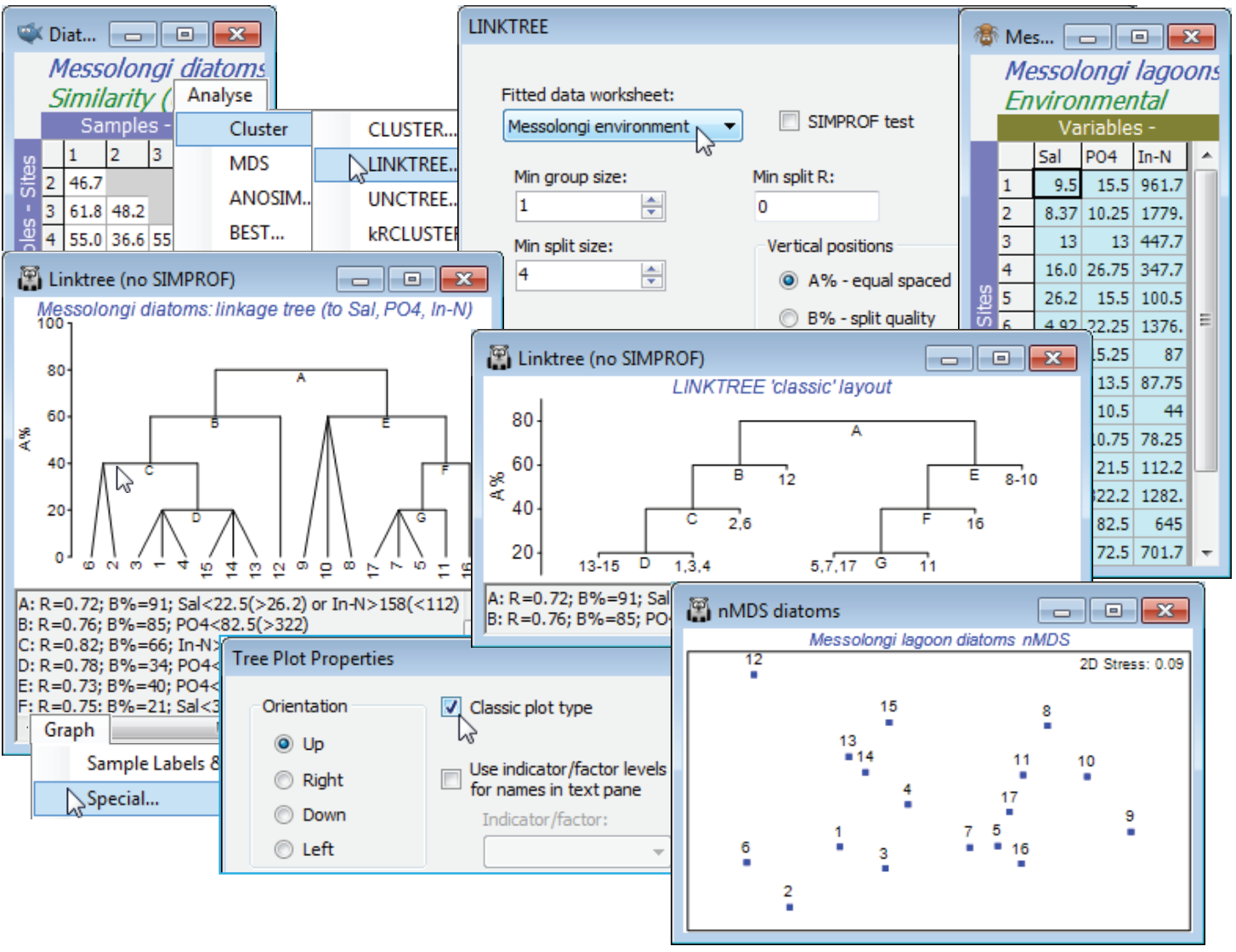
The output is a tree diagram with a text pane below it. The first split (A) in the assemblage data is between sites 1-4, 6, 12-15 (left hand side of the biotic MDS plot shown above, from earlier) and 5, 7, 8-11, 16, 17 (right hand side) – a very natural divide in the ordination (though remember that the procedure works in the high-dimensional space not the 2-d MDS). This has ANOSIM R = 0.72. It is characterised by low or high salinity (Salinity<22.5 to the left, and >26.2 to the right). Note that the inequalities in the text pane (repeated in the results window) are always in this order, with the branch to the left first and the branch to the right following, in brackets. It follows that if the tree is rotated, by clicking on a horizontal bar exactly like a CLUSTER dendrogram, then the inequality in the text pane reverses (the reason for a dynamic text pane rather than just a static results window). Alternatively, the same split A of samples is obtained by choosing In-N>158 to the left and <112 to the right. R is the same whichever variable is used, of course – both can ‘explain’ that biotic split so both are reported. Moving down the left of the tree, the next split (B) divides sites 1-4, 6, 13-15 from site 12, with an R of 0.76, on the basis of PO$_4$ (high phosphate at site 12). Then C splits 2, 6 from 1, 3, 4, 13-15 at R = 0.82, again with two explanations (and convincingly on the MDS), etc. The end result is 8 groups of sites, each determined by a series of abiotic inequalities. Note that R has no tendency to decline/increase on moving down the tree – the ranks are recalculated for each new subset of samples. An absolute measure (B%) which does generally decline with finer group distinctions was given in Section 6 for the analogous UNCTREE plot. This can be used as a y axis for the plot (see over); the A% scale just displays arbitrary equal-spaced steps but that can help the clarity of the ‘classic’ form of linkage/regression tree plot, which is also shown above, and is an option on the Special menu for linkage plots. This menu also allows the plot to be re-oriented, as for a dendrogram, and can replace long variable names in the text pane with short indicator levels.
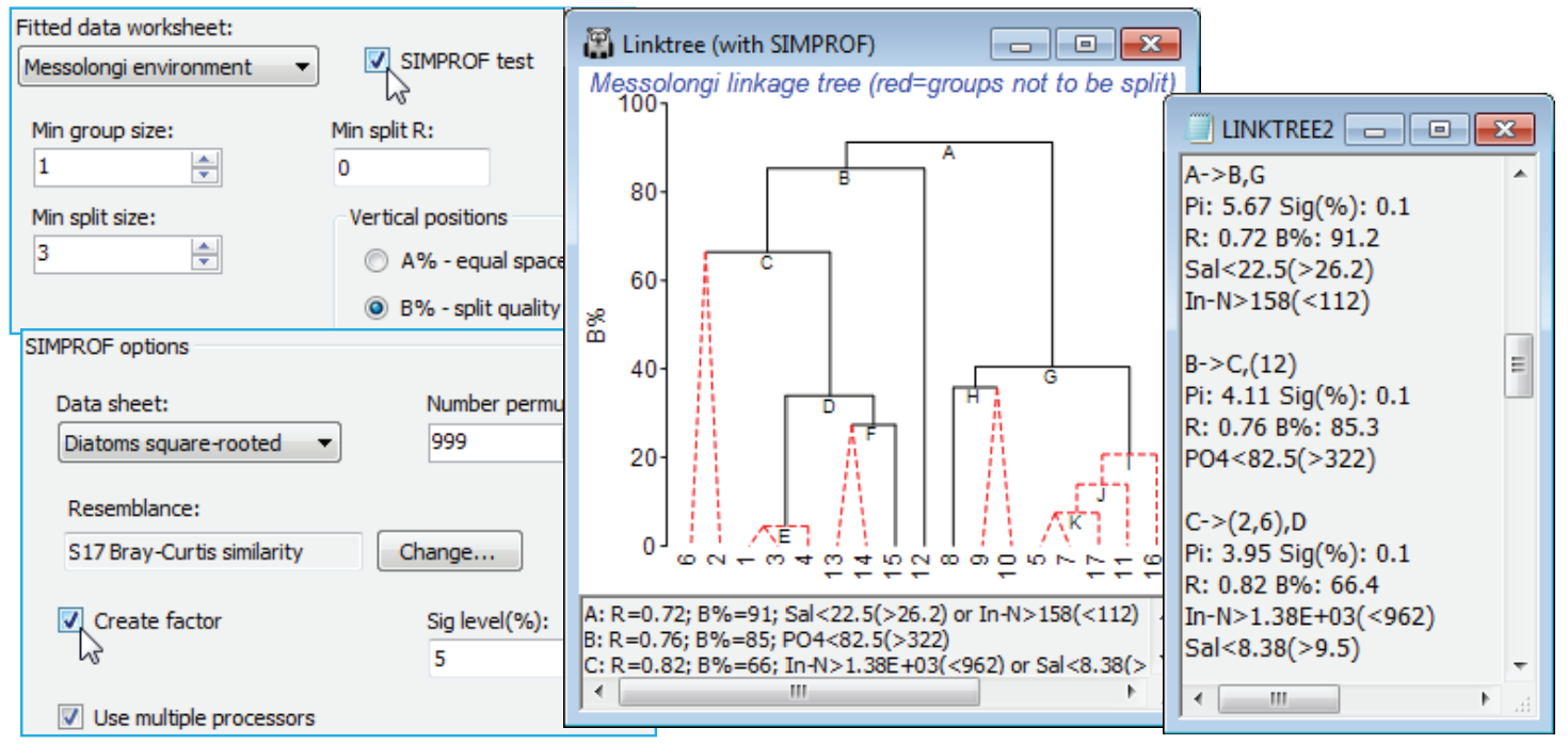
SIMPROF test in LINKTREE
Low values of B% correspond to samples which are rather close together on the MDS plot and the question naturally arises as to whether these samples should be split at all – is there any evidence that the biological assemblages differ among the sites 5, 7, 11, 16, 17? If not, then we should not be seeking an environmental variable which distinguishes two subgroups within them. The SIMPROF test (Section 6) answers this question and provides a statistical basis for interpretation of a further subdivision. The test is the same as used with the unconstrained cluster analyses of Section 6 – the real profile of the biotic resemblances, in rank order, is compared with many repeated profiles from randomly permuting species values across these 5 samples, separately for each species. The test statistic measures departure of the real profile from the mean of the random profiles, and this is set against the range of values it takes for the deviation of (further) random profiles from this mean. A large real $\pi$ implies significance, e.g. if it is larger than all but 49 of the 999 random profiles then homogeneity of the assemblages in this group would be rejected at p$\le$5%, and it is justifiable to interpret the next division LINKTREE makes – the text pane and results window continue to list all divisions permitted by the other stopping rules but the tree branches in red are not significant and it would be unwise to interpret those splits. The results window gives SIMPROF $\pi$ and p values and a factor is created of the SIMPROF groups which can be used to show those groups on an MDS, say.
Run Analyse>Cluster>LINKTREE as before on the diatom resemblances, this time taking (Min split size: 3) so this criterion does not enter – remember SIMPROF can never split a group of two – and (Vertical positions•B%) & (✓SIMPROF test). Look at the entries on the SIMPROF options dialog, but you will probably not need to change any. Since the test is on the biotic data not the environmental, the program steps back in the Explorer tree to find the default (Data sheet: Diatoms square-rooted) whose rows are to be permuted, and the (Resemblance:) specified will be the one used for the active matrix (Bray-Curtis here). You may need to reduce the number of permutations for much larger data problems (this intensive routine exploits available multi-core processing) or just run LINKTREE without SIMPROF tests, and do some selective tests on a few key splits with Analyse>SIMPROF on these selections in Diatoms square-rooted. The plot here shows that (5,7, 11,16,17) do not differ ($\pi \approx$0.95, p<35%) but (1,3,4,13-15) do differ ($\pi \approx$2.3, p<1%) and are split into three interpretable groups. Note also the uneven steps (large and small group differences) in the B% scale, which is now comparable across branches, unlike the equi-spaced A% scale.
Missing data in linkage trees
Note that LINKTREE is able to tolerate some missing data in the abiotic matrix – the piecemeal form of LINKTREE’s conclusions lends itself to analysing what¬ever complete matrix is available locally, i.e. within each created subdivision. But distortions in interpretation from unavailability of explanatory variables in some sets of samples and not others are almost inevitable. A final point to make is that it is always interesting to compare a constrained Cluster>LINKTREE with the un-constrained, but otherwise very similar, Cluster>UNCTREE tree structure. Here, exactly the same divisions are found (and of course confirmed in the same way by the SIMPROF tests). Where there are major differences, this suggests that natural clusters in the samples are not being well identified by the current abiotic suite, perhaps because a key variable is missing (though there are many other possible reasons! – see the discussion on reversals in B% plots in Chapter 11 of CiMC).