14. Further matching of multivariate patterns (RELATE, 2STAGE, BEST + MVDISP)
- RELATE on resemblance matrices
- Model matrix construction
- RELATE hypothesis test
- Seriation (Phuket coral transects)
- RELATE test on two biotic arrays
- 2-way RELATE for seriation
- Seriation with replication
- Other Model Matrix options
- Expanding an (abiotic) data matrix
- Expanded RELATE test (Exe nematodes)
- Expand Samples or Expand resemblances
- Model matrix for 2D Euclidean; Cyclicity (Sea-loch macrofauna)
- 2-way RELATE for cyclicity
- (Leschenault estuarine fish, W Australia)
- Rationale for 2nd stage MDS
- Aggregation & transforms (Morlaix macrofauna)
- Second-stage nMDS (Morlaix macrofauna)
- 2STAGE for resemblance coefficients (Clyde study)
- Conclusions on comparing resemblance coefficients
- 2STAGE for displaying ‘interactions’
- (Phuket coral transect)
- 2STAGE for time series and repeated measures
- (Tees Bay macrofauna)
- (Calafuria macroalgae experiment)
- Other BEST applications
- BVStep stepwise selection
- Species sets ‘explaining’ the overall pattern
- BVStep (Morlaix macrofauna)
- BVStep starting and stopping options
- BVStep from random starts
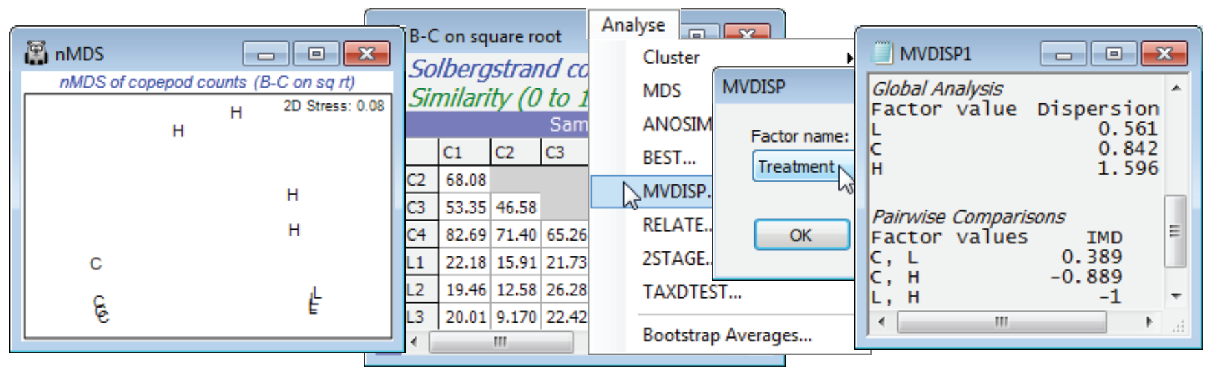
- Multivariate dispersion MVDISP
- (Mesocosm experiment, Solbergstrand copepods)
RELATE on resemblance matrices
The BEST routine in the previous section introduced the concept of measuring how closely related two sets of multivariate data are, for a matching set of samples, by calculating a rank correlation coefficient (Spearman’s $\rho$, Kendall etc.) between all the elements of their respective (dis)similarity matrices. Thus, if the among-sample relationships agree, in exactly the same way in both data sets (e.g. the two closest samples are 3 and 5, the next two closest are 7 and 15, …, and the furthest apart are 6 and 11), then the rank correlation $\rho$ = 1, a perfect match. (These element-by-element correlations of two resemblance matrices are known as matrix correlations or Mantel coefficients, though Mantel – working in epidemiology – defined them with standard Pearson correlations, a less flexible option than rank correlations for our purposes but one which PRIMER now provides). The two resemblance matrices to be compared in this way need not be of biotic and environmental data respectively, but can come from any source: biotic compared with biotic, abiotic with abiotic, biotic with a model matrix, etc. – it is only necessary that they refer to matching sample labels.
PRIMER performs the calculations by the Analyse>RELATE routine, with active window as one of the resemblance matrices to be compared. In fact, RELATE allows the user either to supply the second matrix as another triangular resemblance sheet (the general case) or to specify one of two special cases of simple model matrices, which the routine then constructs for itself. The first is referred to as seriation, where the data is compared to a linear sequence, either in space or time, i.e. the matching coefficient $\rho$ assesses the extent to which samples follow a simple trend: adjacent samples being the closest in species composition, samples two steps apart the next closest, and so on, with assemblages from the first and last samples differing the most. Chapter 15 of CiMC gives more detail on model matrix construction, and draws the clear link between the RELATE test for seriation and the ordered ANOSIM test seen in Section 9 (and described in Chapter 6 of CiMC). RELATE, however, is able to accommodate more complex hypothesised models than the simple serial trends of ordered ANOSIM (with or without replication), e.g. the other model RELATE constructs automatically is simple cyclicity, with the sample relationships thought of as matching those of distances between points placed equidistantly around a circle. A possible context could be monthly samples taken over a full year. With a seasonal signal one might expect adjacent months to be the most similar, months two steps apart less similar etc., but the assemblage structure for later months gradually returns to that at the start, so that Dec and Jan are only one step apart, not 11.
Model matrix construction
Model matrices corresponding to more complicated structures than simple seriation or cyclicity need first to be constructed by the user and then entered to RELATE in the same way as any other resemblance matrix being matched to the active sheet. There are at least three ways of obtaining such model matrices. Firstly, they can be read in directly as a triangular matrix, e.g. as an existing physical distance matrix between the sampling points – there the idea would be to judge how well the community dissimilarities match geographical layout. Secondly, they can be produced from simple x (or x, y or x, y, z) co-ordinates of the sample points by running this 1- (or 2- or 3-) variable data sheet through Analyse>Resemblance, choosing Euclidean distance. For example, if simple seriation (perhaps for an inter-annual time trend) was not already catered for directly in Analyse> RELATE, it could be handled by creating a data sheet with one variable and n samples, of entries 1, 2, …, n, and calculating Euclidean distances – producing a lower triangular matrix with 1’s on the diagonal, 2’s on the first off-diagonal, …, down to n–1 in the lower left corner. And a model distance matrix corresponding to a monthly season cycle would result from the x, y co-ordinates of numbers on a clock face being input to Euclidean distance (again, non-normalised). This will not give model entries which are integers but the distances will be in the correct rank order – which is all that matters for RELATE’s rank correlations). For a geographical layout, enter the metric form of lat/long co-ordinates to Euclidean distance. Thirdly, however, PRIMER helps you to construct model matrices directly from specified factors using Tools>Model Matrix, which is run when the active sheet is the biotic resemblance matrix to be compared with the model. An example given below is of seriation with replication, namely four groups of samples considered to be at points 1, 2, 3, 4 along a line (thus dissimilarity between group 1 and 2 is less than that for 1 and 3, or 2 and 4, and that for 1 and 4 is larger still). This cannot be handled by choice of the seriation option in RELATE because that is only appropriate to single samples at each space (or time) point – here there are replicates in each group, considered to be at distance 0 from each other. Tools>Model Matrix, specifying a numeric factor with appropriate levels 1, 2, 3, 4, will create the correct model.
RELATE hypothesis test
A permutation test can be applied to the matching coefficient $\rho$ between any two resemblance matrices which are independently derived, with all sample labels in the active matrix matched with (some) labels in the supplied resemblances. As remarked in the previous section (in the context of testing for a significant match between biotic composition and a suite of environmental variables), it would not be appropriate to use RELATE on two matrices derived from the same data, e.g. by different transformation or aggregation level on the same set of species abundances. Under the null hypothesis of no relation in sample structure between the two similarity matrices, $\rho \approx$ 0. The null distribution of $\rho$ either side of zero can be obtained by randomly permuting, many times, one (or both) sets of sample labels and recalculating $\rho$, to derive a histogram with which the true value of $\rho$ can be compared. The following example is given in Chapter 15, CiMC (Breakdown of seriation).
Seriation (Phuket coral transects)
The Phuket coral-reef assemblages at equi-spaced positions down an onshore-offshore gradient (transect A) from Phuket Island, were seen previously in Sections 8, 9 and 11. Open the workspace Phuket ws, or if not available open just Phuket coral cover 83-87 from C:\Examples v7\Phuket corals, square-root transform, calculate similarity and create nMDS plots such as that of Section 8, separately for the two years 1983 and 1987. Do this by selecting the 12 samples along the transect in 1983, with Select>Samples>(•Factor levels)>(Factor name: Year>Levels>(Include: 83) – note that Select works in just the same way on a resemblance matrix as a data sheet – then take Tools>Duplicate to make a copy of this smaller resemblance matrix, renaming it B-C 1983. Analyse>MDS>Non-metric MDS with default options, except (✓Fix collapse)>(Metric proportion: 0.05). This is needed to avoid the collapse of the nMDS plot because of the outlying first point on the transect (as seen in Section 8). With Graph>Special>Overlay>(✓Overlay trajectory)>(Numeric trajectory factor: Position), the serial change in coral community over the transect positions is clear. Repeat these steps for 1987, giving resemblance B-C 1987. The choice of (✓Fix collapse) is not necessary here but if you run the nMDS with and without this option you will see that it makes no difference at all to the outcome – the metric proportion of the minimised combined stress function is so small that it cannot influence the plot unless there really is no non-metric information to use, as for Position 1 in 1983, when the metric stress kicks in. (You may want to use the Procrustes routine, Graph>Align Graph on one of these plots, specifying the other as the (Configuration Plot: ) to match to – see Section 8) Align graphs automatically – to see they are indeed identical).
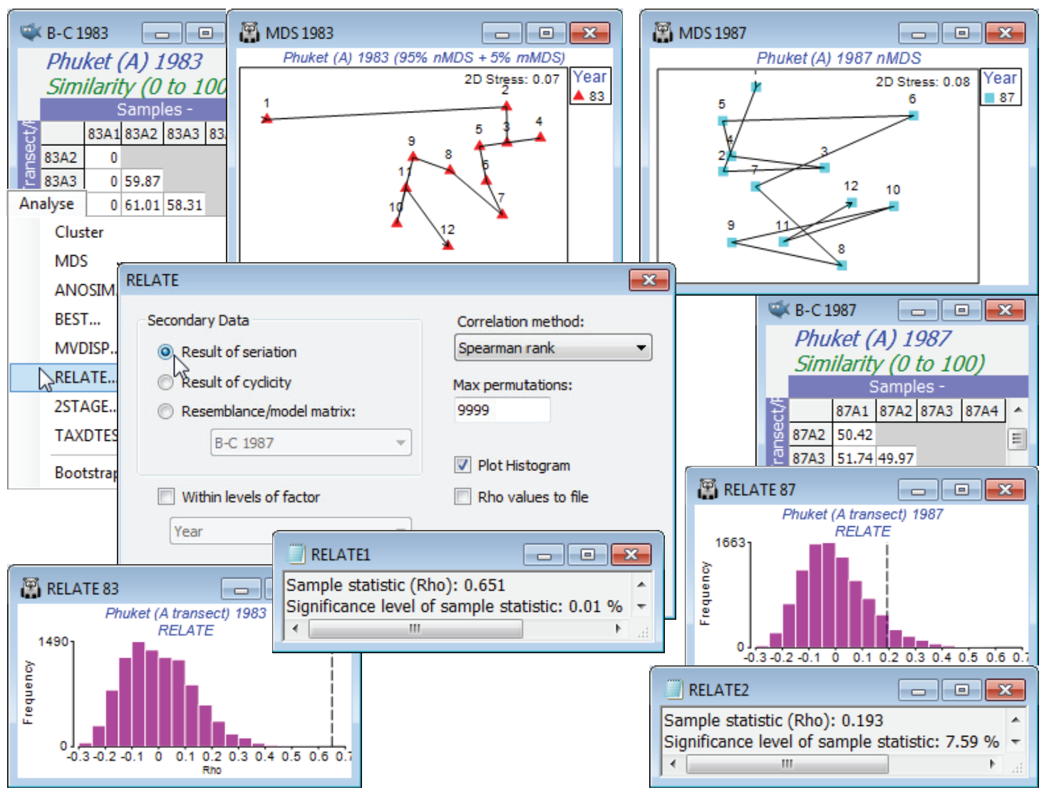
The serial change along the transect in 1983 has largely disappeared in 1987, with sedimentation impact from nearby dredging for a deep-water port. This is reflected in the RELATE tests shown above, with $\rho$ declining from 0.651 to 0.193, e.g. on B-C 1983, Analyse>RELATE>(Secondary Data•Result of seriation) & (Max permutations: 9999), with defaults for the other choices, gives a histogram and results window with observed $\rho$ = 0.651 greater than for any of the 9999 simulated values, so the null hypothesis of no seriation at all ($\rho \approx$ 0) is decisively rejected, p<0.01%. Note that the strong outlier has not wrecked this test, though it somewhat degrades the match to a model of equi-stepped change, as is seen by $\rho$ rising to 0.75 if this first transect position is omitted. [Since we have not provided the factor Position when using the (•Result of seriation) option, the routine has to assume that samples are in the desired equi-stepped serial order – a different order, or a wish to fit unequal steps, perhaps by omission of an intermediate transect sample, must be handled by a Model Matrix.] The $\rho$ = 0.193 for 1987 is more in the body of the null distribution however, and there is no clear evidence in the RELATE test for any serial structure (p $\approx$ 7.5%). In this simple case, there is a very close link with the ordered, unreplicated 1-way ANOSIM test on factor Position (see Section 9), with R (not $\rho$) statistics of R$^{\text Os}$ = 0.655 (p<0.01%) and 0.194 (p $\approx$ 7.0%) for 1983 and 87.
RELATE test on two biotic arrays
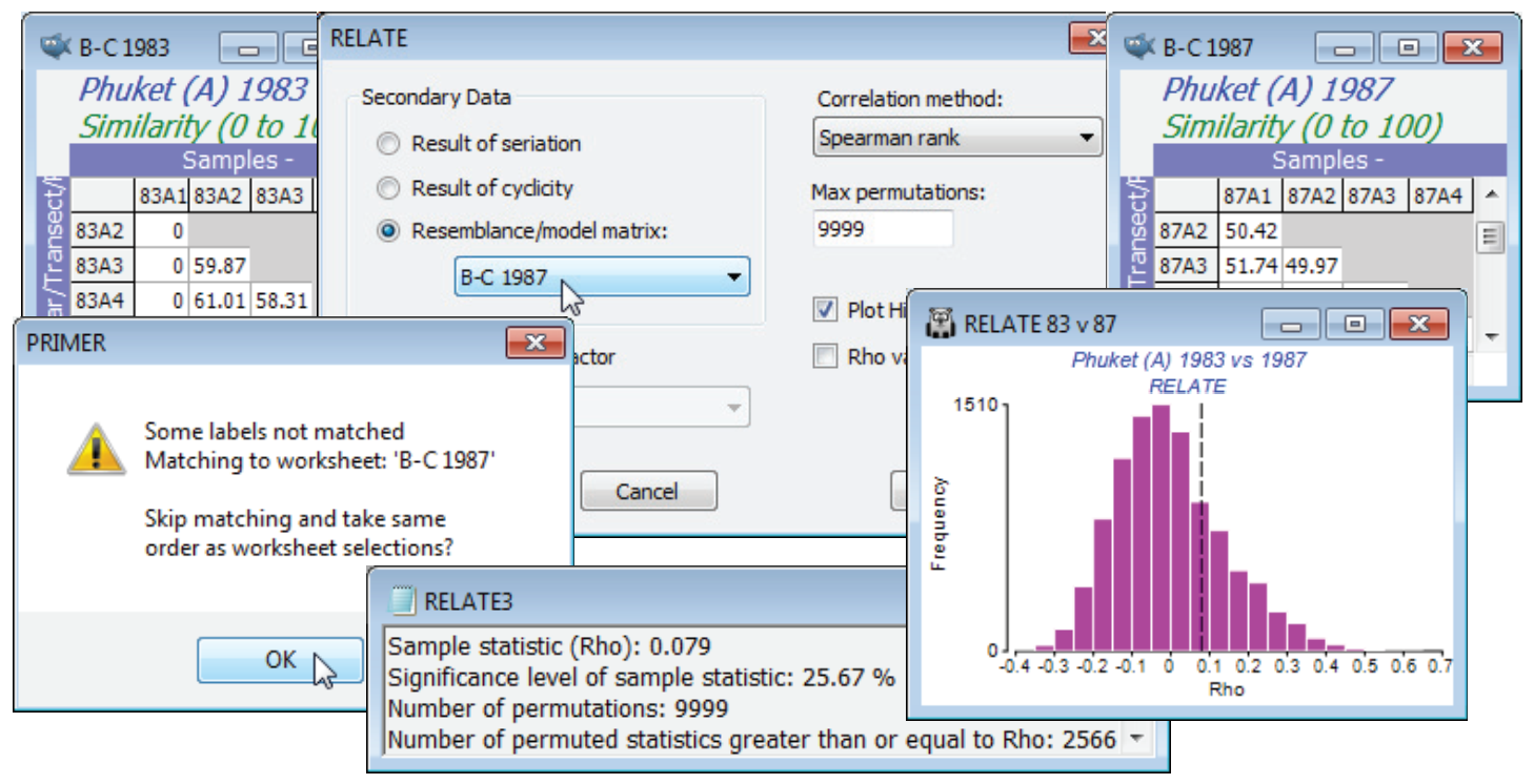
Given the breakdown of the serial gradient structure for 1987, is it now the case that the pattern of change down the transect has nothing at all in common with that for 1983? To answer that question requires a further run of RELATE, but of the two similarity sheets B-C 1983 and B-C 1987 against each other, rather than in comparison with a model matrix. With either as active window, say B-C 1983, take Analyse>RELATE>(Secondary Data•Resemblance/model matrix: B-C 1987). There will be a warning message indicating that the sample labels in the two sheets could not be matched. This issue was raised earlier, in Section 11. PRIMER typically takes label matching very seriously. When linking separate data sheets, as in RELATE or BEST (or the ABC plots of Section 16), the sample order need not be the same in the two matrices – provided it can find all the sample labels of the active matrix somewhere in the secondary sheet, the correct match will take place. However, it is here inconvenient to have to rename both sets of labels (currently 83A1, 83A2, … and 87A1, 87A2, … ) to a common set (A1, A2, …), especially because the data were extracted from a larger sheet, where PRIMER expects the sample labels to be unique! So, this warning message provides an over-ride (take OK) which allows you to skip label matching, and RELATE will pair up the samples in the current order in both sheets. The option will not be offered if the two similarity matrices are not the same size. Instead you will get an error message No labels matched. Cannot match labels, even relaxed. The routine will then need to be run again, having selected the same number of samples in each, and it is your responsibility to make sure they are in the same order!
The results do indeed show that the assemblage patterns down the transect in the two years are totally unrelated. The observed match of only $\rho$ = 0.079 is exceeded by about 2500 of the 9999 permutations under the null hypothesis (p<25%) – the null hypothesis (as always) being that there is absolutely no match in spatial pattern ($\rho$ = 0). Omitting the outlier (Position 1) from both series, makes little difference to this conclusion, $\rho$ now dropping still further to 0.016 (p<44%).
2-way RELATE for seriation
A new feature in PRIMER 7 parallels that discussed for the BEST analysis of the previous section, namely a secondary factor is supplied, e.g. (✓Within levels of factor ), which turns this into a 2-way RELATE test. The matching statistic $\rho$ – whether that is to simple seriation, simple cyclicity or a supplied resemblance/model matrix – is calculated only on samples within the levels of this secondary factor, and the $\rho$ values averaged to give the overall test statistic. The permutations for the test are similarly constrained to be within the strata of this eliminated, secondary factor.
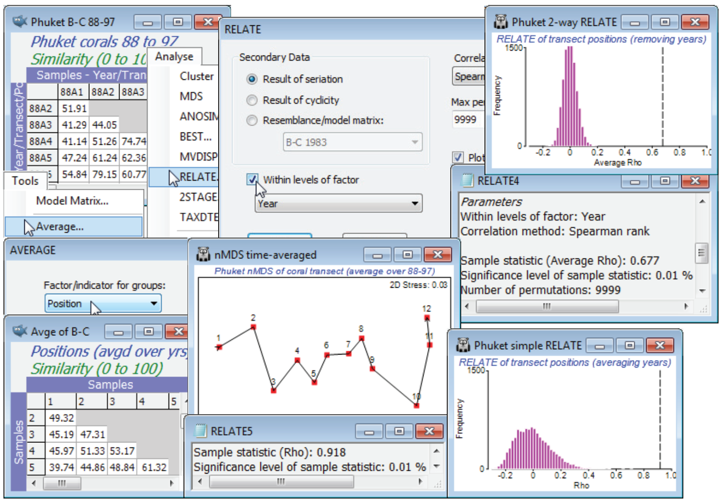
In the current Phuket ws workspace, open (if necessary) the data file Phuket coral cover 88-97, and run the same root-transform and similarity as above, for these 12 transect positions $\times$ 7 years – a period with no known new stressors on the coral reef. Running RELATE on this similarity matrix, under the simple (•Result of seriation) model, and for (✓Within levels of factor Year ), removes the inter-annual differences by calculating a simple trend statistic $\rho$ across the transect positions, separately for each year, and then averaging those. (Note again that since we have not supplied the Position factor in setting up the test, the routine presumes that the samples for each year are in the desired serial order in the matrix). This is now a test statistic for the null hypothesis of no serial community change along the transect in any year, giving a large average $\rho$ of 0.68, and obviously an overwhelmingly significant result (p<0.01%). An alternative test would have been to average the samples over the years for each transect position (by Tools>Average using factor Position, on either the transformed data or the similarity matrix) and perform a simple seriation test on the 12 samples of the resulting matrix. As the nMDS plot for these averages shows, there is a very steady time-averaged gradient of change along the transect with RELATE statistic $\rho$ = 0.92 (p<0.01%). However, the histogram of the null distribution is seen to take values up to 0.3 or 0.4, in contrast with that for the 2-way RELATE test for which values larger than about 0.1 will be significant. In other words, 2-way RELATE is the more powerful test – by eliminating the year differences rather than averaging over them it has many more permutations and this could be important for testing very short runs of serial change (an averaged test with 5 transect positions has only (5!/2) = 60 distinct permutations, at best an $\approx$2% level test, and 4 positions is not viable, with 12 permutations).
The above example was met in Section 9, under the 2-way ordered, unreplicated ANOSIM test, and there is again a very close affinity of the average $\rho$ statistic with the average ANOSIM R$^{\text Os}$. In fact, there is no advantage here in using the 2-way seriation RELATE test – the equivalent ordered ANOSIM test is marginally preferable (see Chapter 6 in CiMC on ANOSIM for ordered factors). However, ordered ANOSIM is constrained to the simple serial model, whereas 2-way RELATE comes into its own, later, when we move to other model matrices, e.g. seriation for a time series where the times are not equally spaced, and we wish to allow for this in computing the statistic (though in most cases that will make very little difference because of the rank nature of the tests) or, more importantly, when the model is not serial but cyclic, or based on a supplied resemblance matrix from abiotic variables, perhaps. This takes us back to the 2-way BEST construction of the previous section – matching to an environmental resemblance matrix, having removed a categorical factor. The difference of 2-way BEST from 2-way RELATE, of course, is that between any global BEST test and an equivalent RELATE test – the former allows for the selection bias in repeating abiotic variable choices until the best match is found, whereas the latter assumes a single fixed set.
Save the workspace Phuket ws, which will be returned to later in the context of 2nd stage analysis.
Seriation with replication
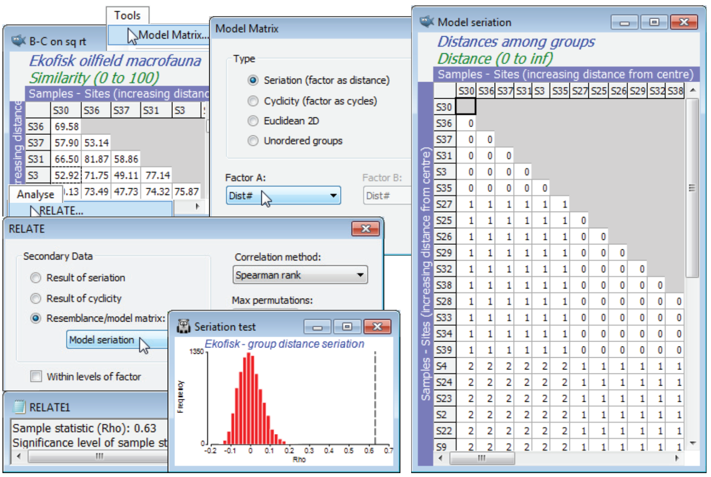
Return to the macrofaunal data set from the Ekofisk oilfield, with workspace Ekofisk ws last saved in C:\ Examples v7\Ekofisk macrofauna in Section 9, following an ordered 1-way ANOSIM test (with replication) on the similarity matrix B-C on sq rt from data Ekofisk macrofauna counts. This used factor Dist#, which is the numeric form of the four groups of sites at different distances from the oilfield, $\sim$logarithmically spaced (1$\equiv$D:<250m; 2$\equiv$C: 250m-1km; 3$\equiv$B: 1-3.5km; 4$\equiv$A:>3.5km). The rationale for an ordered test here was discussed in Section 9 (and Somerfield PJ, Clarke KR, Olsgard F 2002, J Anim Ecol 71:581-593), namely the improved power but more limited generality in testing the null H$_0$: no differences against an ordered alternative H$_1$: A$\rightarrow$B$\rightarrow$C$\rightarrow$D, rather than the unordered alternative H$_1$: A, B, C, D differ (in ways unspecified). Those authors, and previous versions of PRIMER, did not use the generalised (ordered) ANOSIM statistic – which is new to PRIMER 7 – but used the analogous RELATE statistic $\rho$ between the biotic resemblances and a model matrix for seriation with replication. This is a model matrix which Analyse>RELATE does not handle internally in the (•Result of seriation) option – that is restricted to simple seriation with no replication – but which can be simply constructed from the active matrix B-C on sq rt, using Tools>Model Matrix>(Type•Seriation (factor as distance)) & (Factor A: Dist#). [The factor Dist, splitting the sites into alphabetic levels D, C, B, A, will not work here because distances cannot be calculated between names]. A model matrix is generated – rename this Model seriation – having blocks of 0’s down the diagonal (sites within a distance group are considered 0 distance apart), then off-diagonal blocks of 1’s then 2’s then 3’s (sites in groups 1 and 2 are 1 unit apart, in groups 1 and 3 are 2 units apart etc.). Again with B-C on sq rt active, run Analyse>RELATE>(Secondary data• Resemblance/model matrix: Model seriation), giving $\rho$ = 0.63 (p<0.01%), providing clear evidence of group differences, with large $\rho$ confirming the strongly ordered gradient away from the oilfield.
Other Model Matrix options
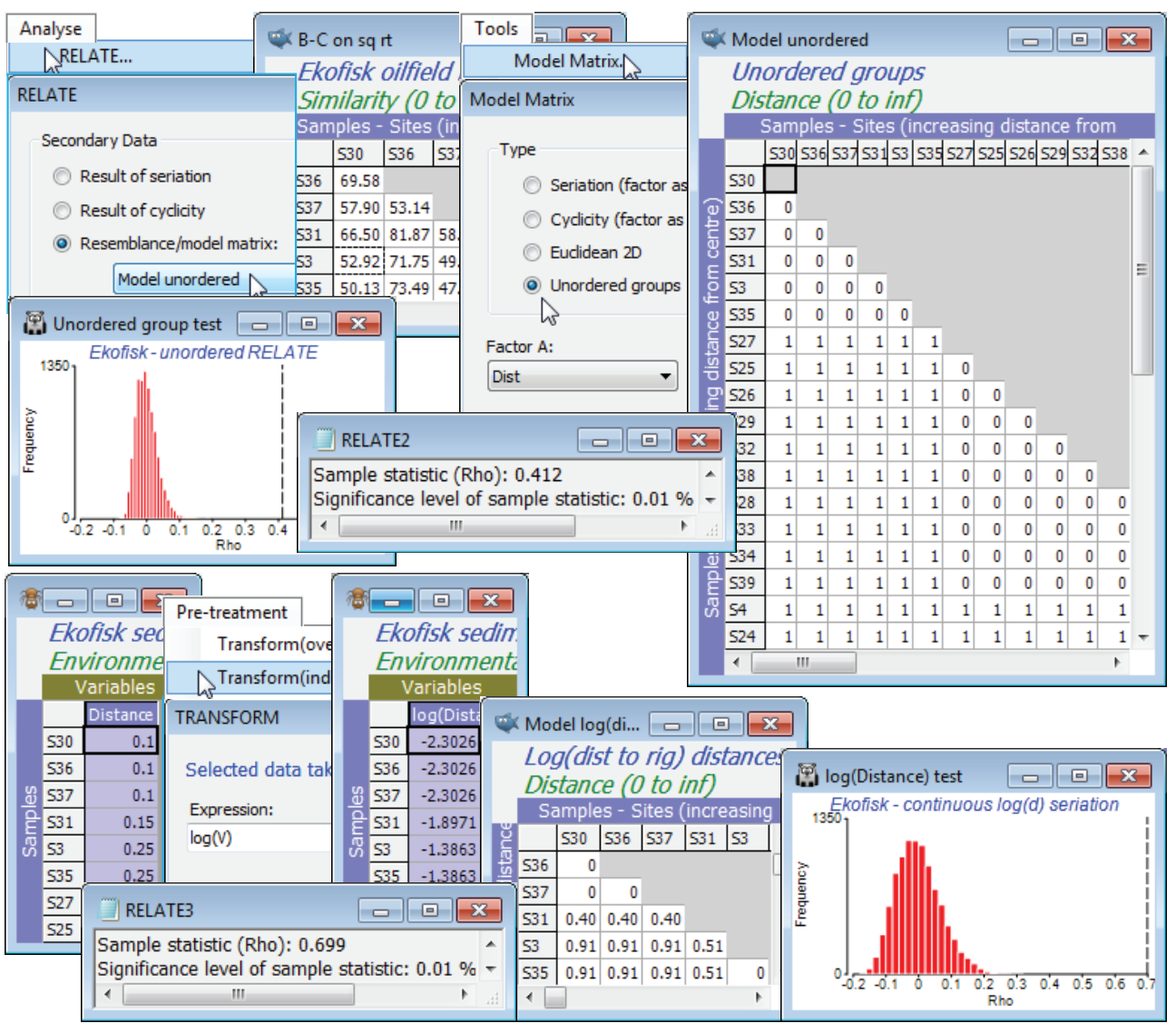
The conclusion is, of course, consistent with the different, but closely-related, ordered ANOSIM statistic R$^{\text Oc}$ = 0.67 (p<0.01%), calculated in Section 9. It is relatively easy to show algebraically that the unordered ANOSIM statistic – here R = 0.55, with p<0.01% again – is exactly equivalent (see Chapter 6 of CiMC) to a RELATE $\rho$ test with model matrix having 0’s in the diagonal blocks (samples within the same group) and 1’s elsewhere (samples in different groups), i.e. all groups are considered equally different from each other. Such a model matrix can be constructed by Tools>Model Matrix>(Type•Unordered groups) & (Factor A: Dist) – or (Factor A: Dist#), since it no longer matters whether an unordered factor is supplied as numeric or alphabetic. This test returns $\rho$ = 0.41, again strongly significant, naturally, but much lower than the seriation statistic $\rho$ = 0.63.
So far we have not seen anything that could not have been slightly better carried out with ordered and unordered ANOSIM tests (in the sense that the statistic upper limit of +1 is attainable for R$^{\text O}$ but not for $\rho$ – see Chapter 6 of CiMC – and because ANOSIM will allow pairwise comparisons among the groups). But another possible model here which we would like a comparison with – one which can only be handled by RELATE – is to ignore the arbitrary distance group structure and RELATE the biotic similarities to the distance matrix calculated from (log-transformed) distances of each site to the oilfield centre. (The log transform reverses an exponentially decreasing dilution curve of contaminant concentrations with distance). The raw distances are in the first column in the abiotic sheet Ekofisk environment, the Distance variable (you may need to Select>All to find it!). Highlight and select just this column, log transform it by Pre-treatment>Transform(individual)> (Expression: log(V)) and Analyse>Resemblance>(Measure•Euclidean distance), renaming the result as Model log(distance) and inputting it as the secondary matrix to an Analyse>RELATE on B-C on sq rt. The result is again significant, naturally, but arguably demonstrates an even stronger gradient of assemblage change with this model of continuous (logged) distance from the oilfield, $\rho$ = 0.70 (p<0.01%). This model matrix could also have been created by copying the log(Distance) entries into a factor log(D) under the B-C on sq rt resemblance sheet and running Tools>Model Matrix>(Type•Seriation (factor as distance)) & (Factor A: log(D)). Save and close Ekofisk ws.
Expanding an (abiotic) data matrix
A RELATE test could equally well have been carried out between the Ekofisk community pattern and a matching (abiotic) resemblance matrix computed not from the surrogate for increased impact – the nearness of the sites to the oil-field centre – but from a set of contaminant levels themselves, as measured at each site. (For the tests of this section, we assume that this set is fixed – we are not allowing selection of a subset of contaminant variables which appears to best match the observed community pattern, i.e. the BEST(Bio-Env) procedure of the previous section. RELATE tests do not allow for this selection bias). All that is necessary for a simple RELATE test of community to a fixed environmental variable suite is that we have one-to-one matching of the abiotic data to each community sample. The active sheet for Analyse>RELATE would logically be the biological resemblance coefficient and the (Secondary data•Resemblance/model matrix) would typically be Euclidean distance on a selectively transformed then normalised abiotic data matrix (though the test would be the same if the matrices were the same size and entered in the opposite order). But where the community data consists, for example, of replicate samples at a number of sites, and the abiotic matrix consists of a single value for each of the suite of variables (which may itself be an average over replicate abiotic measurements, but not matched to the community replicates) then the abiotic matrix needs to be expanded to the same dimensions as the biological matrix, and its entries repeated appropriately. This is achieved by the Tools>Expand Samples routine operating on the active matrix of the abiotic data. It is not cheating – at least, not necessarily! It depends on what is then done with the expanded matrix. If we pretend that the repeated readings are independently measured – by running an ANOSIM test on them for example – then of course we are heading for trouble. But in this context the requirement is an expansion of the Seriation with replication test of the previous page – we want to test the null hypothesis that there are no differences among sites against the specific alternative that there are such differences and that they are determined by the environmental structure among sites (in statistical parlance we condition on this, so the situation becomes no different than if we were testing against a design structure, e.g. seriation or treatment levels). So, the test is no longer of seriation with replication but of a more complex environmental relationship among the sites, but it has the same characterising feature that the resulting RELATE $\rho$ value will capture both whether the sites differ at all and whether they do so in a way that matches the (multivariate) abiotic relationships among sites. A high $\rho$ can only be obtained if both are true. An alternative would be to average up the community replicates to the site level and carry out a simple RELATE test to the abiotic data at that level. However, this might have very little power if there are few sites and it misses the important comparison of whether $\rho$ for this specific alternative is greater than $\rho$ for the unordered test (the 1-way ANOSIM-type model matrix of 0’s and 1’s).
Expanded RELATE test (Exe nematodes)
As an example of Tools>Expand Samples on a data matrix (or Tools>Expand on a resemblance matrix, since the expansion can be equally well achieved either before or after the computation of Euclidean distance in this situation) we shall use the Exe nematode study and the form of the data met in Section 9, in which the 19 sites from different environmental conditions around the Exe estuary were sampled 6 times through one year (with just 6 missing samples spread over several sites, i.e. 108 meiofaunal core samples in total). The biotic matrix is Exe nematodes bi-monthly in C:\Examples v7\Exe nematodes, comprising abundances of 182 species (its time-averaged form was used extensively in Section 8). Also open the abiotic data, Exe environment, which we have not encountered here but which is used as a motivating example for the BEST routine in Chapter 11 of CiMC. It consists of 6 sediment-based environmental variables, postulated to be structuring the communities of free-living nematodes, and recorded as relevant to each site over the full year of sampling: median particle diameter, depth of the water table, depth of the blackened H$_2$S (anoxic) layer, height up the shore (this was an intertidal study), % organics and the interstitial salinity. The environmental data therefore has only 19 samples, which are labelled with the site numbers (1-19). Importantly for the Expand routine, those labels need to be exactly the same as the levels for the site factor which is defined for the 108 samples of the Exe nematodes bi-monthly biotic matrix.
The biotic samples do have a time (i.e. seasonal) structure, in that they are all collected bi-monthly – factor time, with levels A, B, C, D, E, F in common for each site. The time factor will be ignored, however, for the purpose of this illustration and the (up to) 6 values used as replicates for each site. This is not unreasonable, since they will represent both the spatial and temporal variability at that site through the year (providing a conservative estimate of the true residual variability) and it was seen earlier – in Section 9 for sites 12-19 but true also for all sites – that 2-way crossed ANOSIM (without replication) fails to find significant evidence of a seasonal effect at all.
The Exe nematodes bi-monthly biotic matrix requires fourth-root transformation before the usual similarity calculation (resemblance B-C 4rt), and the nMDS plot for all 108 samples, with symbols as the site and labels removed (from Graph>Sample Labels & Symbols), shows clear differences among sites. The unordered RELATE test – equivalent to unordered 1-way ANOSIM but giving a $\rho$ test statistic which we can compare with the expanded abiotic test – is obtained by running on the active B-C 4rt sheet: Tools>Model Matrix>(Type•Unordered groups) & (Factor A: site) to give the Unordered model. Then, again on B-C 4rt, Analyse>RELATE>(Secondary data•Resemblance/ model matrix: Unordered model) gives a Spearman rank statistic of $\rho$ = 0.33 (p<0.01%) – though highly significantly different from zero (and thus confirming site differences), $\rho$ is not large.
Expand Samples or Expand resemblances
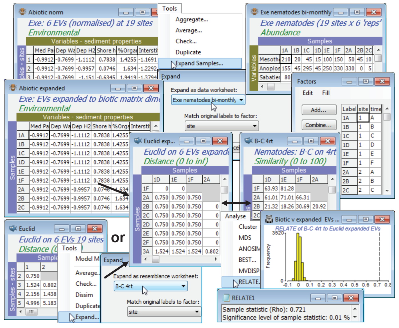
The Exe environment matrix does not seem (from Plots>Draftsman Plot or Histogram Plot) to contain notable outliers and can safely be used without transformation of individual variables. It does however need Pre-treatment>Normalise Variables – rename it Abiotic norm. To expand this data matrix to the dimensions of 108 samples $\times$ 6 variables, with Abiotic norm as the active sheet take Tools>Expand Samples>(Expand as data worksheet: Exe nematodes bi-monthly) & (Match original labels to factor: site). The fourth-root form of the biotic data matrix could equally well have been used in place of the original nematode sheet – what is needed from it is the size of expanded matrix needed, and the structure of samples over the sites, from the factor site whose levels 1, …, 19 are matched up with the labels 1, ..., 19 of the normalised environmental sheet. The expanded environmental matrix is then entered to a Euclidean distance resemblance calculation, to give Euclid expanded. The same construction can be achieved by first taking Euclidean distance on the Abiotic norm data matrix, to give a resemblance matrix renamed Euclid, and then entering this as the active matrix in Tools>Expand>(Expand as resemblance worksheet: B-C 4rt) & (Match original labels to factor: site) to obtain exactly the same model (abiotic) matrix Euclid expanded.
Now with active sheet B-C 4rt a further run of Analyse>RELATE>(Secondary data•Resemblance /model matrix: Euclid expanded) gives a much larger $\rho$ of 0.72 (highly significant, of course, at p<0.01% for the 9999 permutations of this run), indicating the very good fit of the individual bi-monthly samples to the alternative model of sites differences, structured by these abiotic variables.
Model matrix for 2D Euclidean; Cyclicity (Sea-loch macrofauna)
The other two Model Matrix options are (Type•Cyclicity (factor as cycles)) and (Type•Euclidean 2D). The latter simply calculates, for example, distance between samples in a geographic layout when the x, y co-ordinates of the sample points are not held in a separate (environment-type) data sheet but as numeric factors in the biotic data. The corresponding model for sample locations in a 1D layout, given by a single factor, is just the (Type•Seriation) option, or equivalently, set up a Factor B with the same level (e.g. 1) for all samples and take the (Type•Euclidean 2D) option.
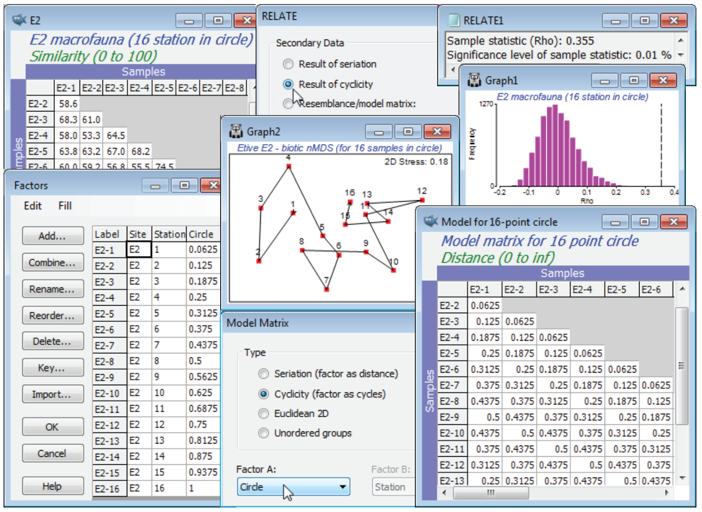
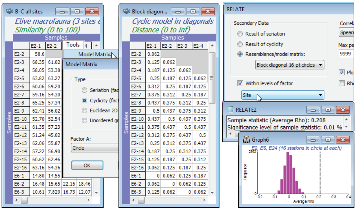
The (Type•Cyclicity (factor as cycles)) option in Model Matrix needs a numeric factor over the range (0, 1), representing the distances round a circle, where 0 and 1 are at the same point (or think of these as the angles at which those points are set, ranging over 0 to 1, not 0 to 360). The obvious examples of such data are in a time-series over a full seasonal cycle (see shortly), or a diel or tidal cycle, but we shall start with an unusual spatial example from studies described by Gage JD 1972 Mar Biol 14:281-297 (and analysed in a multivariate way by Somerfield PJ & Gage JD 2000 Mar Biol 136:1133-1145), of subtidal macrobenthos in Scottish sea-lochs. The subset of these samples used here is from three sites in Loch Etive, at each of which 16 samples (factor Stations, 1-16) were taken approximately around the circumference of a 100m diameter circle at equal spacing. Over all three places (factor Site, E2, E6, E24) counts were made of a total of 186 species, in data file Etive macrofauna counts, directory C:\Examples v7\Sea-loch macrofauna. Open the data and select, for the moment, just the 16 samples from Site E2, by Select>Samples>(•Factor levels)>(Factor name: Site)>Levels>(Include: E2) & (Available: E6 & E24). On fourth-root transform and Bray-Curtis similarities, run the nMDS ordination and test the null hypothesis that there are no differences in communities at these 16 stations against the alternative of a circular structure (their spatial layout) with Analyse>RELATE>(Secondary data•Result of cyclicity). For simple cyclicity such as this, with equal spacing, no replication at each point, and an assumption that the stations are in correct order round the circle, the routine creates the model internally, and an explicit construction of the model matrix is not needed. However, it is instructive to create the model externally, from active sheet of the biotic similarities of the 16 samples, using Tools>Model Matrix>(Type•Cyclicity). The supplied (Factor A:) is not the Stations levels 1-16, but these numbers divided by 16, held in the factor Circle – in general the points, e.g. times, may not be equally spaced and the routine must be told how the start and end of the sequence relate to each other, hence the restriction to (0,1). The same RELATE test now results from using this cyclic model under (•Resemblance/model matrix: Model for 16-point circle), giving weak but still significant cyclicity ($\rho$= 0.355, p<0.01%).
2-way RELATE for cyclicity
A 2-way RELATE version of the above test where there are no replicates, and the cyclic factor under test is actually nested within a ‘nuisance’ factor whose effect we want to remove, is given by reverting to the full data sheet for the Loch Etive macrofauna samples: Select>All and recompute the fourth-root transform and Bray-Curtis similarities, as B-C all sites, which now has 16 samples in a circle for each of the three sites E2, E6 and E24. Testing for a match with the circular spatial layout of stations, simultaneously at all three sites, whilst eliminating the inevitable differences in community composition for these three locations using 2-way RELATE, should give a still stronger test of the null hypothesis of no community differences within sites against this specific alternative.
As before, the model matrix is constructed by Tools>Model Matrix>(Type•Cyclicity) & (Factor A: Circle), run on B-C all sites, giving a model distance matrix (rename it Block diagonal 16-pt circles) in which only the block diagonals of the stations within sites will be sensible in this nested case (and which is all that RELATE uses) because, for example, station 1 at E2 and station 1 at E6 have nothing in common. On B-C all sites, Analyse>RELATE>(Secondary data•Resemblance/ model matrix: Block diagonal 16-pt circles) & (✓Within levels of factor Site) gives an averaged $\rho$ statistic across the three sites of 0.21, still strongly significant – note the tighter spread of the null histogram (c.f. Graph1 above) because of the simultaneous testing. The lower value than for the E2 test alone suggests weaker effects at E6 and E24, which is seen in separate (1-way) cyclic tests.
More usually, the cyclic factor under test (often time) is crossed with a second factor (often space), whose effect we want to eliminate for our time test. The 2-way RELATE test structure is the same as for the above nested case however, and a more typical example is now given of a cyclic four-seasons series recorded for several regions, with the added complexity of replication within each of the cells of this 2-way layout. Though the structure is that of a 2-way crossed ANOSIM, this case is not covered by running an ordered ANOSIM test because, of course, the time factor is cyclic and not serial – an appropriate model matrix therefore needs to be created as an input to RELATE.
(Leschenault estuarine fish, W Australia)
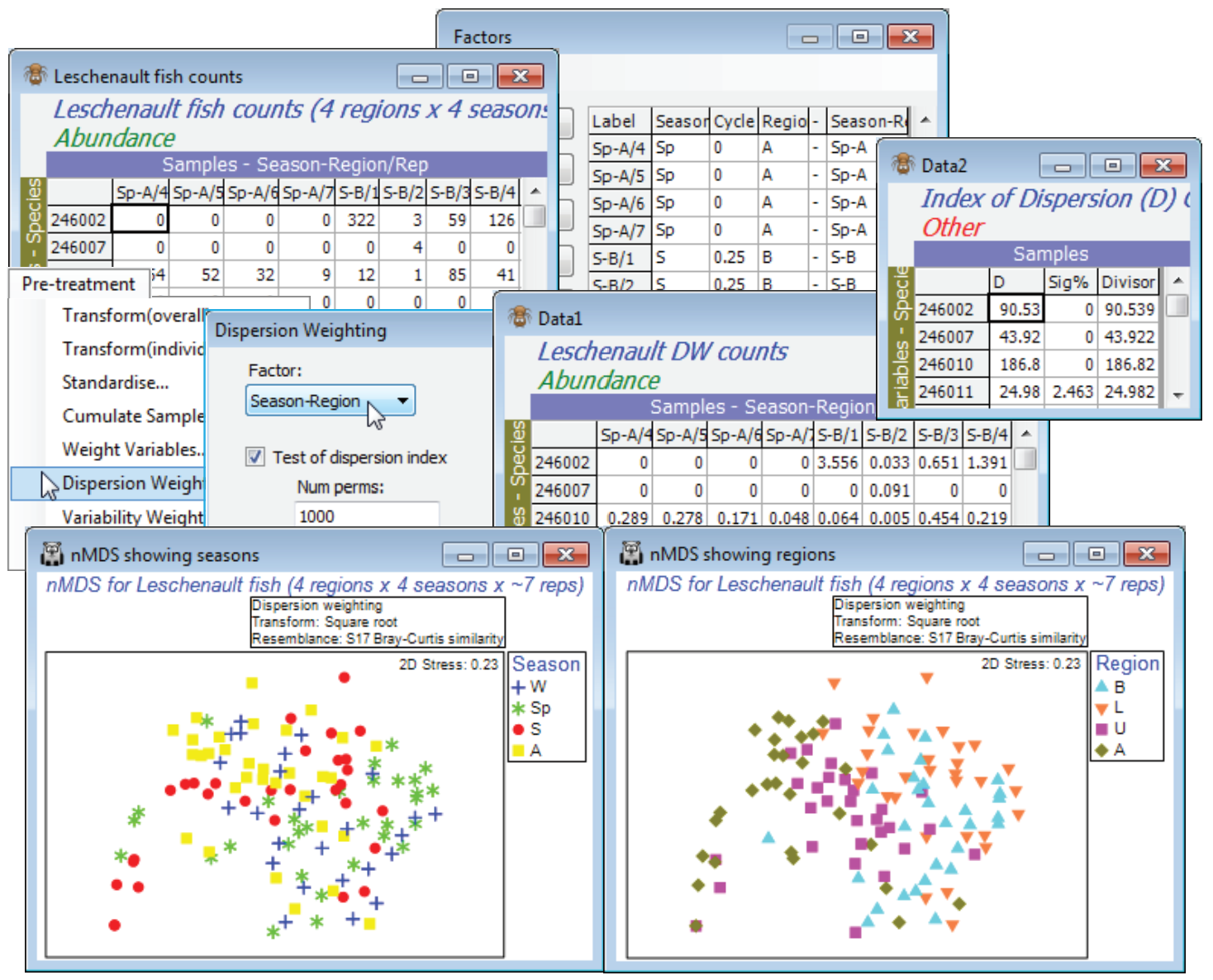
Veale L et al 2014 J Fish Biol 85: 1320-1354 describe trawl sampling for nearshore estuarine fish in the Leschenault estuary of Western Australia, over 4 regions (B - Basal, L - Lower, U - Upper, A - Apex of the estuary) and 4 seasons (Sp - Spring, S - Summer, A - Autumn and W - Winter). The data set used for this illustration has been somewhat simplified and consists of 6-8 replicate 21.5m seine net samples reflecting both inter-annual and spatial variation within each of the 16 region $\times$ season combinations. Due to the location of freshwater inputs and restricted exchange with the ocean, the estuary has a salinity gradient which increases from the basal (mouth) through lower and upper regions to the estuary apex. Counts are given of 43 fish species (with numerical ID), file Leschenault fish counts in C:\Examples v7\Leschenault fish. Close the above workspace and open this file, with factors Season and its (0, 1) numeric form Cycle (0, 0.25, 0.5, 0.75), then Region.
As often with fish data, over-dispersion of counts (shoaling) can be substantial for some species, their erratic counts over replicates giving them too much weight in a community assessment, and Clarke KR, Tweedley JR, Valesini FJ 2014 J Mar Biol Ass UK 94: 1-16 show that a good strategy for such fish data is often pre-treatment by Dispersion Weighting (Section 4 and Chapter 9, CiMC) followed by mild transformation (square root). So, take Edit>Factors>Combine>(Include: Season & - & Region), where - is just a hyphen separator in all rows, to create a new factor Season-Region whose levels identify the groups of replicates from the 16 conditions. Use this in Pre-treatment>Dispersion Weighting>(Factor: Season-Region) & (✓Test of dispersion index) &(✓Stats to work-sheet), and the latter sheet shows that counts of some species are, indeed, heavily downweighted by an index of dispersion D of up to nearly 200. However, Plots>Shade Plot (Section 4) or Wizards> Matrix display (Section 10) on the dispersion-weighted data still show that the contributions to the resemblance matrix will come from relatively few of the species, so take a further Pre-treatment> Transformation(overall)>(Transformation: Square root). Now calculate Bray-Curtis similarity on this full set of 119 samples (B-C on root DW), and an nMDS ordination with symbols for Region, and duplicated with symbols for Season, show a great deal of replicate variability and consequent high stress, but also some evidence for effects of both factors.
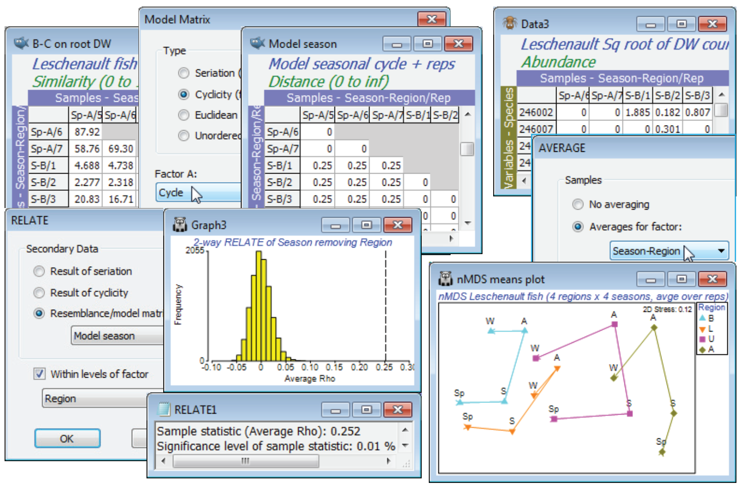
Unordered two-way ANOSIM with factors Region and Season is perfectly viable and will provide pairwise comparisons, though there is a good case for 2-way ANOSIM with an ordered Region factor, because of the salinity gradient and the geographical ordering of the regions B, L, U and A (note that a numeric factor would need to be created to capture this order). Such a serial order is not appropriate for Season, however, with the cyclic relationship of its levels (the factor Cycle, with Sp = 0, S = 0.25, A = 0.5, W = 0.75; though Sp could equally well have been coded 1, of course). The optimum test of Season therefore creates a model structure from B-C on root DW with Tools> Model Matrix>(Type•Cyclicity) & (Factor A: Cycle) to give Model season and tests it by 2-way RELATE on the active sheet B-C on root DW with RELATE>(Secondary data•Resemblance/ model matrix: Model season) & (✓Within levels of factor: Region). The resulting match to a cyclic seasonal pattern in each region – under the 2-way model, separately calculated then averaged to give $\rho$ = 0.25 – is low but this simply reflects the high replicate variability and therefore the strong overlap of the communities in the different seasons for the same region. Importantly, this value is highly significantly different from zero, as the histogram shows (p<0.01% since 9999 permutations were again used). This certainly justifies an nMDS means plot, averaging the replicates for the 16 conditions (4 seasons $\times$ 4 regions). As we have seen, there are several possible ways to do this – averaging the replicates of the original counts, or the dispersion weighted and transformed data, or the similarities (or, in PERMANOVA+, using distances among centroids in the high-d PCO space). Here, take the second method, Tools>Average>(Samples•Averages for factor: Season-Region) on the transformed DW data matrix, then recalculate the Bray-Curtis similarities and the nMDS, on which display symbols as Region as labels as Season using Samp. Labels & Symbols, and overlay split trajectories using Special>Overlays>(✓Overlay trajectory:Cycle)>(✓Split trajectory:Region). Both the consistent community change up the estuary (B,L,U,A) and the matching seasonal cycles are evident. (Lines logically joining W and Sp, as in Fig. 15.12 of CiMC, can be added by copying and pasting the plot into Powerpoint, or similar software, where it can be ungrouped to Microsoft drawing objects and manipulated as vector graphics). Close the Leschenault workspace.
Rationale for 2nd stage MDS
As seen above, the $\rho$ statistic, which rank correlates the elements of two similarity matrices, can provide a very useful and succinct summary of the extent of agreement between two ordinations (or, to be more precise, of agreement in the high-dimensional multivariate data underlying these low-dimensional plots). Often, many such pairwise comparisons are made; for example, a single set of data may first be aggregated to a range of taxonomic levels (species, genus, family, …), then analysed under a range of pre-treatments: standardisations (none, by species or samples, and by maximum or total); other taxon weightings (e.g. dispersion weighting); then transformations (none, square root, 4th root, log, pres/abs), etc. Many ordination plots result and it is reasonable to ask how much the multivariate pattern changes as a result of these various decisions. What are the important choices? Does it matter whether the data are only identified to family rather than species level, or is the difference this makes completely dwarfed by the changes resulting from choosing to look at common to mid-abundance species (none or square root transform) or concentrating more on the less-common species (4th root or presence/absence)? Or is it the choice of a resemblance coefficient (from the 40 or so in Section 5) that really dictates the conclusions? It can be difficult, and arbitrary, to assess this just by looking at the range of different ordinations produced, though at least we can exploit the $\rho$ statistic to give quantification of the agreement in multivariate pattern for any pair of choices. But when there are many choices, even a set of $\rho$ values between pairs does not become a succinct enough description (considering only two types of choice, there are 20 different ordinations from 5 transformations and 4 taxonomic levels, thus 190 $\rho$ values between them!).
The key step here is to realise that $\rho$ itself can be regarded as a similarity measure, taking values near 1 if two multivariate patterns are highly similar and near zero if they bear no relation to each other. So, the triangular matrix of $\rho$ coefficients between all pairs of ordinations can be entered into the MDS routine, to obtain what PRIMER calls a 2nd stage MDS plot (an MDS of MDS’s, if you like!). The $\rho$ coefficient is not a distance-like measure (it can take small negative values and has a fixed upper limit) so it is unlikely to be turned into an ordination distance by a straight line through the origin on a Shepard plot, so again nMDS rather than mMDS seems appropriate This is based on the rank orders of the $\rho$ values, therefore catering naturally with the potential for small negative $\rho$ values – these just become patterns that are even less like each other than random re-arrangements, and in practice large negative values are not observed. The resulting second-stage nMDS plot thus gives a succinct summary in a 2-d picture, often with small stress, of the relationship between the multivariate sample patterns under the various choices. The 2STAGE idea was introduced in this context by Somerfield PJ & Clarke KR 1995 Mar Ecol Prog Ser 127:113-119 and further explored by Olsgard F, Somerfield PJ, Carr MR 1997 & 1998 Mar Ecol Prog Ser 149: 173-181 & 172: 25-26, and is also covered extensively in Chapter 16 of CiMC, including the examples below.
Aggregation & transforms (Morlaix macrofauna)
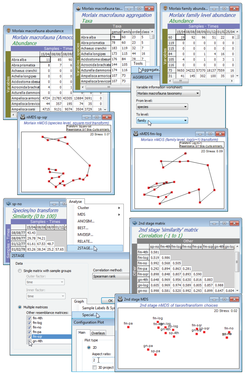
Chapter 10 of CiMC gives several examples of aggregating species matrices to higher taxa – using the Tools>Aggregate routine – and the effect this has on the resulting multivariate (and univariate) analyses. We shall illustrate this with the benthic macrofauna data from the sediments of the Bay of Morlaix, sampled at 21 times over April 1977 to February 1982, covering the period of the Amoco-Cadiz oil tanker wreck in March 1978. This was last seen in Section 10 and introduced in Section 8 where the species-level nMDS (and tmMDS) showed the strong community change following the oil-spill and the subsequent partial recovery, with the re-establishment of a clear seasonal cycle. Open that workspace, Morlaix ws in C:\Examples v7\Morlaix macrofauna, or if unavailable, open the species data matrix Morlaix macrofauna abundance and the variable information (aggregation) file Morlaix macrofauna taxonomy. Calculate a couple of aggregation and transformation options, computing Bray-Curtis similarities and running nMDS, e.g. contrast plots for species-level, square-root transformed and family-level log transformed data (similarities sp-sqr and fm-log). The latter requires, on the active sheet Morlaix macrofauna abundance, Tools>Aggregate>(Variable information worksheet: Morlaix macrofauna taxonomy) & (From level: species) & (To level: family), followed by Pre-treatment>Transform(overall)>(Transformation: Log(X+1)) and resemblance etc. as usual. On the resulting nMDS plot, take Graph>Samp. Labels & Symbols to remove labels and the (✓By factor) on symbols, and Special>Overlays>(✓Overlay trajectory: time). A similar pattern is seen to that for the species-level root-transformed case but showing an apparently greater degree of recovery. One possible explanation for this is seen in the line plots (coherent curves) of Section 10 – the effect of the highly abundant Ampelisca species prior to the spill, whose numbers crash and do not recover well, is more heavily down-weighted with the severe log transformation.
Second-stage nMDS (Morlaix macrofauna)
The illustration below has calculated all combinations of species (sp), genus (gn) and family (fm) level data, under no transform (no), square-root (sqr), fourth-root (4th), log(x+1) (log) transforms and reduction to presence/absence (pa), with similarity sheets sp-no to fm-pa. [Actually, all these have already been calculated for you, as PRIMER format *.sid files in the directory C:\Examples v7\Morlaix macrofauna\Morlaix similarities, and you can open as many of them as you need into the workspace in one batch by File>Open, highlighting them all and taking Open]. With one of these as the active matrix (it does not matter which – one of the very few routines for which that is true), run Analyse>2STAGE>(Data•Multiple matrices)>(Other resemblance matrices: ✓fm-4th & ✓fm-log & ✓fm-no & …) & (Correlation method: Spearman rank). This returns a second-stage resemblance sheet of matrix correlations $\rho$, all of which are positive, with some very close to 1 (e.g. species and genus level under no transform; 4th root and log transforms for any of the taxon levels, etc.), indicating robustness of the conclusions to those particular choices. Now run nMDS on this matrix to obtain the 2nd stage MDS plot – note that the plot below has had its boundary shape changed with Graph>Special>Main>(Plot type•2D)>(Aspect ratio: 2.0). The main conclusions are that: transform choice and taxonomic level tend to have orthogonal effects (transformations run across the page, taxon levels run up the page); transform choice generally makes a larger difference to the outcome than taxon level (the exception being between 4th root and log, which are more or less equivalent – log being more severe than 4th root on very large abundances but less severe than 4th root for small counts); the difference between taxonomic levels increases with the severity of the transformation. The latter is to be expected, since untransformed analysis tends to be dominated by a handful of species with the largest abundances – when these are in different genera or families their contribution is unchanged by aggregation. Save Morlaix ws for later this section, and close it.
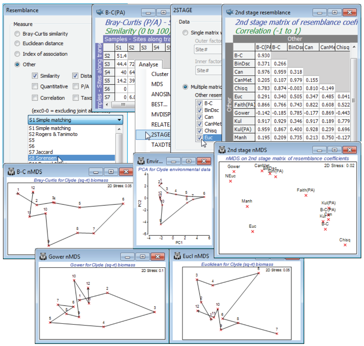
2STAGE for resemblance coefficients (Clyde study)
The technique of 2nd stage plots has also been used (Clarke KR, Somerfield PJ, Chapman MG 2006, J Exp Mar Biol Ecol 330: 55-80) to examine the effects of different resemblance coefficient choices on a samples analysis, scaling this in relation to the effects of differing transformation (and, by extrapolation, taxonomic level). The environmental data from the Clyde sewage dump-ground study were used extensively in Sections 11 and 12 but, for this example, open the macrofaunal data C:\Examples v7\Clyde macrofauna\ Clyde macrofauna biomass into a new workspace, and deselect the all-blank species (there are about 20 of them retained in this sheet because they have non-zero counts in the abundance matrix but their total biomass is too small to weigh). You can do this by Select>Variables>(•Use those that contribute at least 0.001%), then take a square-root transform (Biomass sq-rt). Always starting from this matrix, produce a wide range of distances and (dis) similarities using Analyse>Resemblance>(Analyse between•Samples) & (Measure•Other)> (✓Similarity) & (✓Distance/dissimilarity), selecting one coefficient at a time from the resulting list, e.g. S1 Simple matching, S8 Sorensen (i.e. Bray-Curtis P/A), S13 Kulczynski (P/A), S26 Faith (P/A), S15 Gower, S18 Kulczynski (quant), Canberra similarity exc 0-0, D7 Manhattan distance, D10 Canberra metric, D16 Chi squared distance, Binomial Deviance (scaled) and (•Bray-Curtis similarity) and (•Euclidean distance) from the main dialog, the latter both with and without normalisation of the species variables. [You should read the discussion in Section 5 and in Chapter 16 of CiMC on the suitability or otherwise of some of the coefficients in the full list, for non-count data]. With (say) S8 Sorensen as the active sheet, Analyse>2STAGE>(Data•Multiple matrices), ticking the check boxes for all the rest, and running nMDS on the resulting 2nd stage matrix. Look also at individual MDS plots for some measures with differing effect, in comparison with the contaminant gradient (the multivariate analysis for which – a PCA – is shown in Section 12). Crosses have been used for points in these plots, by changing the symbol type temporarily in the Samp. Labels & Symbols>(Default>Symbol:) dialog or, changing the global default by Tools>Options>Graphs.
Conclusions on comparing resemblance coefficients
Clarke KR, Somerfield PJ, Chapman MG 2006, J Exp Mar Biol Ecol 330: 55-80 discuss this analysis (and that for several other data sets) in more detail, but to pick out just four general points:
a) These 2nd stage plots have common features, irrespective of the actual data set, e.g. coefficients which are in what they term as the ‘Bray-Curtis family’ (including quantitative measures: S17, S18 & Ochiai (quant), matched by pres/abs measures: S8, S13, S14; also Canberra similarity exc 0-0) tend always to cluster on the 2nd stage plot, i.e. produce similar multivariate conclusions, and radically differ from Euclidean distance, even more so when the latter is normalised.
b) Choice of coefficient is much more crucial to a multivariate analysis than transformation (which itself is more important than taxonomic level – see earlier); this is apparent here by noting the relative proximity of the Bray-Curtis and Bray-Curtis P/A (Sorensen) points, and the Kulczynski and Kulczynski P/A points, on the 2nd stage plot (the first of the pair uses a mild square root, and the second is on presence/absence data – the most severe transform possible).
c) The inference of similarity from joint absences for coefficients such as Euclidean distance, S15 Gower etc., has a dramatically adverse effect on their performance in describing gradients of assemblage change where there is a turnover of species (i.e. pres/abs data is informative); this is clear from the above (1st stage) MDS based on Euclidean distance, which places site 6, at the centre of the dumpground, close to the extreme ends of the transect, 1 and 12, when 6 has no species in common with either! Similarity is deemed higher because they share absent species. The radical effect of counting (or not) joint absences is also clear here from: the separation of the Canberra metric from Canberra similarity (the only difference is an adjustment for double zeros, Section 5), and the way the plots splits left, right (counts 0-0, ignores 0-0), with the Faith coefficient intermediate since it counts joint absences, but with less weight than joint presences.
d) Another key feature which separates out the behaviour of coefficients is whether they implicitly or explicitly standardise (or normalise), and whether over samples or species. Chi-squared distance does both, removing all differences in total abundance between samples and also having a divisor of the total abundance of each species across all samples – low density species can be given very heavy weight, leading to problematic behaviour. Normalised Euclidean and Gower also have a species (but not sample) standardisation, giving rare and common species equal weight.
Close the workspace – we shall start a clear workspace next time we meet this data (Section 15).
2STAGE for displaying ‘interactions’
A very different way of using 2nd stage matrices is best accessed through the alternative entry option in the dialog box for 2STAGE, namely to specify a single similarity matrix with factors defining a 2-way crossed layout of samples (e.g. of sites and times), and allow 2STAGE to select the sub-matrices on which to calculate the second-stage correlations. To motivate this, return to the Phuket coral data at the start of this section, in which the spatial pattern of assemblage change over an onshore-offshore transect was compared for two years, 1983 and 1987. The rank correlation (Spearman) between the two Bray-Curtis similarity matrices underlying these profiles was only $\rho$ = 0.08, indicating a poorly matching sequence, the conclusion being that the sedimentation from dredging for a deep-water port in 1986 and 87 had disrupted the spatial pattern of the assemblages. In fact, that study has data from 13 years over 1983 to 2000 (the merged file for which was created in Section 11). This period included a further potentially disruptive event in 1998, a prolonged high pressure anomaly creating a period of low sea levels, increasing the frequency of desiccation. If the transect patterns for all pairwise sets of years are now matched, a correlation matrix of $\rho$ values is produced, which is the second stage matrix. These ‘similarities’ between years can be input to an MDS or clustering to give a visual summary of the inter-annual changes, not of the community as such (i.e. not of the average assemblage, or the assemblage at one fixed point on the transect – that would be a first-stage MDS) but of the internal pattern of assemblage change along the transect. Years which are anomalous in terms of their spatial pattern should stand out as outliers on this 2nd stage MDS or 2nd stage cluster analysis. If the inter-annual differences do not disrupt the internal spatial structuring but simply, for example, increase the abundance of all species down the transect in some years, relative to others, then the 2nd stage plot will show nothing whatsoever – that type of signal will be seen in a (1st stage) plot of yearly changes in the community, when averaged over the whole transect. In a sense, what the 2nd stage plot does is to remove ‘main effects’ of years (to use familiar univariate terminology) and concentrate on ‘interactions’, the changes in the internal spatial gradient for some years compared with others. This example is now implemented but is also discussed, along with other examples, in Clarke KR, Somerfield PJ, Airoldi L, Warwick RM 2006, J Exp Mar Biol Ecol 338: 179-192, and at the end of Chapter 16 of CiMC.
(Phuket coral transect)
Open the workspace Phuket ws, of coral cover for the Ko Phuket transect A, in C:\Examples v7\ Phuket corals, or if not available, open the data files Phuket coral cover 83-87, 88-97 and 98-00, and Tools>Merge them (as in Section 11), taking the defaults to produce the full inter-annual series, Phuket coral cover 83-00. This has 156 samples, in a 2-way crossed design split into 13 years, with 12 positions along the onshore-offshore transect (look at the factors Year and Position with Edit>Factors). Create the similarity matrix for all 156 samples as previously: Bray-Curtis on square-root transformed data, renaming it B-C all. On this, take Analyse>2STAGE>(Data•Single matrix with sample groups)>(Outer factor: Year) & (Inner factor: Position) & (Correlation method •Spearman rank) to produce the 2nd stage matrix, renamed 2stage Resem. On this, run Analyse>CLUSTER and Analyse>MDS, drawing clusters on the MDS using Graph>Special>(✓Overlay clusters) – see Section 8 – with slice at resemblance ($\rho$) of 0.2. Contrast this 2nd stage plot with the (1st stage) MDS of years, averaging over the transect positions with Tools>Average for factor Year (on original or transformed data, or perhaps from the similarity matrix B-C all – a case can be made for all three methods here!), then re-run the MDS. Although testing is impossible in this case, it is clear that this first stage plot of the year ‘main effect’ is less sensitive in picking up the impacts of sedimentation (86 and 87) and desiccation (98) than the second stage analysis, concentrating on the consistency over years of the spatial pattern along the transect (‘interaction’ effects).
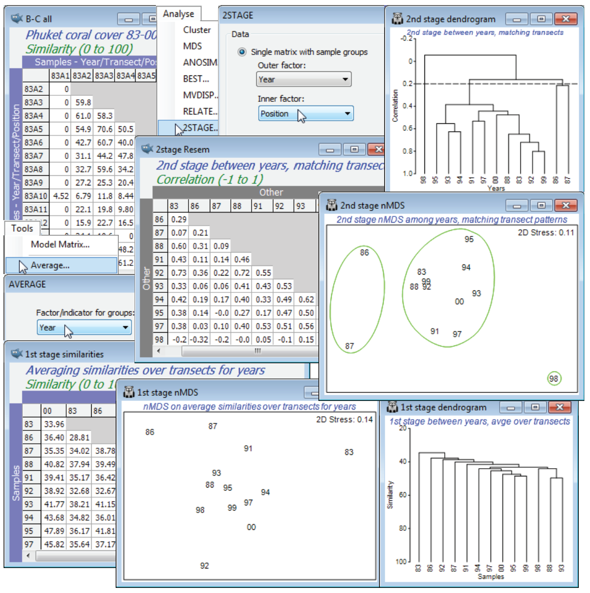
Save and close the Phuket ws. A more natural context for 2nd stage analysis is that of temporal studies, in which similarities in the time course are being compared across sites under different conditions, and this can give rise to cases where tests for this rather general concept of ‘interaction’ between time and space are possible, as in the time series for Tees Bay macrofauna now examined.
2STAGE for time series and repeated measures
In the context of a 2-factor design, PRIMER makes a 2nd stage matrix very simple to produce but it is less easy to understand what it represents! The structure requires that the factors divide the data into a 2-way layout with no replicates in each cell; the inner factor specifies the patterns to match (spatial, for the Phuket data) and the outer factor is the one displayed (temporal, above). Note that, because of the symmetry of two-way crossed designs, these could be reversed, thus the Phuket data could have matched the inter-annual patterns at each point on the transect. This would remove the ‘main effect’ of differences in (time-averaged) assemblages along the transect, and concentrate on anomalous transect positions – those for which the relationship among years differs. The Clarke, Somerfield, Airoldi & Warwick 2006 paper, referred to above, discusses two further examples in which Analyse>2STAGE is able to match temporal patterns to produce a spatial second-stage matrix. Both have a natural hypothesis testing framework, which extends to repeated measures designs, usually considered problematic even in univariate studies. An inter-annual time series (1973-96) for subtidal macrobenthos, at two sites in each of four different areas in Tees Bay, UK, was met in Section 9, and will be exemplified here, and a repeated measures recolonisation study on macroalgae at Calafuria in the Ligurian Sea (the non-repeated measures data from which was seen in the ANOSIM section) is also discussed in detail as the last example in Chapter 16, CiMC.
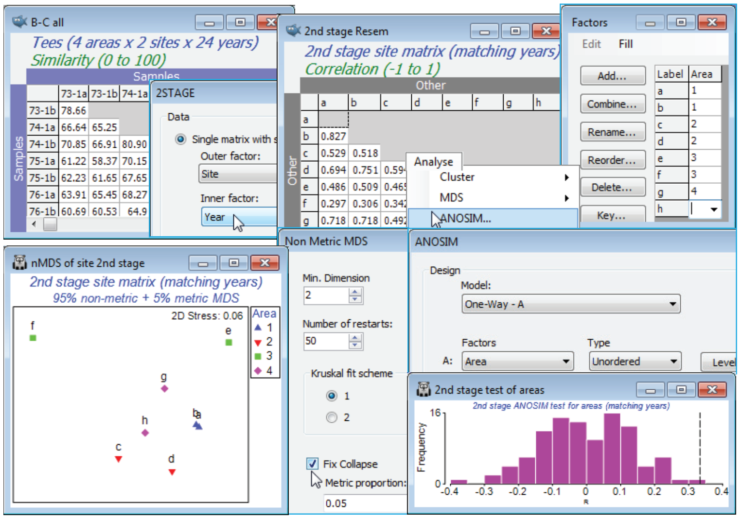
(Tees Bay macrofauna)
The workspace Tees ws was saved in Section 9; if not available open the data Tees macrobenthic abundance from C:\Examples v7\Tees macrobenthos and recalculate Bray-Curtis similarity on the 4th-root transformed abundances for all 192 samples (B-C all), with structure of 4 areas (1-4) in each of which the same 2 sites (a,b; c,d; e,f; g,h) were sampled in September over 24 years (1973-96), with each sample a pool of a consistent number of benthic grabs. A question of interest here is whether the areas show the same inter-annual patterns – as might be expected if they are primarily influenced by wide-scale climatic variation – or whether local factors, such as the proximity of the plume from the Tees estuary to some areas (with the inevitable local changes in an industrialised estuary) result in different time trajectories in different areas. This can be addressed by calculating, on B-C all, a second-stage matrix for the 8 sites, by Analyse>2STAGE>(Data•Single matrix with sample groups)>(Outer factor: Site) & (Inner factor: Year). On the resulting sheet 2nd stage Resem, set up the simple Area factor (by Edit>Factor>Add) with entries 1,1,2,2,3,3,4,4 – the sites are the replicates – and run 1-way ANOSIM on factor Area, and nMDS plots of the 8 points (you will need the ✓Fix collapse option, Section 8). The ANOSIM is not a test for different assemblages over the areas – that is inevitable given the spatial range – but removes those, and shows that the temporal variations for each area (from different baseline communities) are not the same (R = 0.33, p<1%).
(Calafuria macroalgae experiment)
The Calafuria macroalgal recolonisation experiment monitored the same physical rock patches over one year, having first cleared the (subtidal) rockface. Replicate patches were tracked for 8 different ‘treatments’, namely different times of year for the clearance. The 2STAGE analysis matches the recolonisation time patterns of all replicates, and a 1-way ANOSIM on the 2nd stage matrix tests whether different treatments give different recolonisation profiles (which they do). The individual time points in the recovery sequence cannot be assumed independent, since the same rock patch is returned to bi-monthly – this is repeated measures. But the 2nd stage analysis treats that inter-dependent time sequence of recovery as a single experimental unit, in effect. It becomes a single point on the 2nd stage MDS plot and a single replicate in the 2nd stage ANOSIM, independent of other replicates (other rock patches), and thus gives a fully valid test. An equally valid alternative would have been to throw away the intermediate recovery times and just analyse the assemblages at one year after clearance (which is the data analysed in Section 9, which also introduces a lower level to the design, of plots within areas, under the different treatments). In fact, the second-stage analysis is more incisive here because it allows the whole recovery profile to be assessed rather than solely its end point – but different hypotheses are being tested, and both are of interest.
Other BEST applications
Another situation employing rank correlation ($\rho$) between two resemblance matrices is the BEST (Bio-Env) routine of Section 13, where the biological similarity matrix (‘response’) describes the among-sample relationships of the full community and the secondary data sheet (‘explanation’) is of environmental variables. Subsets of the latter variables were taken, and among-sample distances computed for each subset and correlated with the biotic similarities, the search being for a variable set that maximises $\rho$. However, there is nothing in the construction of BEST which limits its use to species similarities and environmental matrices. Either or both of these two sheets could be from biotic or abiotic samples – the user needs only to specify a resemblance measure which is relevant for the type of data in the secondary data matrix. A number of possibilities can be envisaged. In what might be termed Env-Bio, subsets of species could be selected which best characterise the environmental gradient defined by a specified set of abiotic variables, or best match a simple model structure, e.g. the seriation distance matrix for n equally-spaced points on a line, as in the Phuket corals transect example earlier in this section (“which species define the serial gradient along the transect?”). Or for samples which have an a priori (unordered) group structure, a relevant model matrix of distances was seen to consist simply of 0’s (within groups) and 1’s (among groups). An Env-Bio analysis in that case would search for subsets of species which, in combination, best split the samples into those pre-defined groups – a rather different form of SIMPER analysis (Section 10) acting on all the groups at once, rather than selected pairs. It is equivalent to optimising the ANOSIM R statistic, PRIMER’s preferred measure of group separation in high-d space. [We saw ANOSIM R used in the same way earlier, Sections 6 & 13, in searching for optimal subdivisions of samples in divisive clustering, though there the set of species was fixed and the sample divisions selected, and here the sample groups are fixed and the set of species is being searched over. It should be stressed again that having selected an optimal species set, it is totally invalid to re-test the groups with a simple ANOSIM test! The strong selection bias effect is allowed for, however, in the global BEST test of Section 13, so that when sample groups are fixed a priori the BEST test could be used to justify interpreting the selected optimal species subset as ‘better than chance’.]
A further generalisation would allow ordering on the groups, e.g. for the seriation with replication model matrix described earlier in this section. There the idea would be to select the subset of species which best characterise an ordered group structure of community change, i.e. lead to both good separation of the groups from each other and in their pre-defined order (e.g. as in the distance groups for the Ekofisk oil-field study). A similar use of variable selection to best match a priori ordered groups was given by Valesini F et al 2003. Est Coast Shelf Sci 57: 163-177, under what might be termed an Env-Env scenario, since the variables were beach morphology characteristics, and thus required a distance-based resemblance calculation, such as normalised Euclidean. Other natural applications of this type might include the selection of biomarkers to best display a given impact gradient determined by tissue chemistry, the selection of morphometric measurements to best characterise known species or sub-species categories (unordered groups or ordered clines) etc., again supplemented by the global BEST test, to allow for the selection bias when testing overall significance of the ‘explanation’ (but see the important reservations expressed in Chapters 11 and 12 of CiMC on the extent to which correlative-type links of species to environmental variables, biomarkers to tissue contaminants etc., are ever demonstrated to be causal).
BVStep stepwise selection
There is one fundamental problem with applying BEST (Bio-Env) in many of the above scenarios: the number of variable combinations from the active matrix that must be considered in a full search increases exponentially with the number of variables. For p variables, there are (2$^p$ – 1) combinations, and this is prohibitive for p more than about 16 (c. 65,000 combinations). Searching across all subsets of species from a typical community matrix will therefore usually prove impossible. The (•BVSTEP) option under Analyse>BEST instead carries out a stepwise search: the best single variable is selected (maximising the matching coefficient, $\rho$); this is retained and the best variable to add to this is selected (maximising $\rho$); these two are retained and a third variable is added, and so on, resulting in a declining number of combinations to be considered at each step. This is called forward selection. BVStep also carries out backward elimination: starting with all the variables included, the one that decreases $\rho$ least, when omitted, is dropped from the set, and this elimination process repeated. In fact, as is common with stepwise procedures elsewhere (e.g. in multiple linear regression), BVStep implements both forward and backward steps successively, so that after each addition of a variable by forward selection, the current set of variables is scanned to see if any of the other variables can now be eliminated. (The analogy with stepwise multiple regression is not perfect, note, because there the residual sums of squares always decreases as more variables are added – here the $\rho$ value may go up or down, giving a natural optimisation). It follows, however, from the fact that only a small fraction of the possible combinations are considered, that the routine can become trapped in a non-optimal maximum, just as nMDS can get trapped in a local minimum of the stress function (Section 8). The answer is the same as for MDS – repeat the search from a different starting position. So, the BVSTEP dialog lets the user specify how many random restarts are required (choose as many as are computationally feasible). Each restart is from a different, randomly chosen, combination of the variables – experience suggests that it is better not to start with too large a number because it can be difficult to shed extremely sparse variables that neither help nor harm the best solution, so the default is set at 6. Chapter 16 of CiMC gives more detail on the operation of the forward/backward stepping algorithm and the application below.
Species sets ‘explaining’ the overall pattern
The main application area for the BVStep routine introduced by Clarke KR & Warwick RM 1998, Oecologia 113: 278-289, is what might be termed Bio-Bio, namely searching for subsets of species whose resemblance matrix best matches that of another (fixed) set of species. One can envisage this used on different faunal (taxonomic- or trophic-based) groups to elucidate potential interactions but the most obvious context is when the two biological matrices are from the same data. That is, the input similarity matrix is computed from the full set of species, and the secondary data sheet from which species are selected is the same full species data. Now, the idea is not to maximise $\rho$, since it can always be made equal to 1 by choosing a subset which is the full set of species, but to find the smallest possible subset of species which, in combination, describe most of the pattern in the full data set. ‘Most’ in this context is taken to be a conventional, and somewhat arbitrary, $\rho$>0.95. Once $\rho$ gets to about this level, two multivariate patterns (e.g. as seen in 2-d ordinations) are effectively indistinguishable, and would not lead to different interpretations.
The procedure can be thought of as a generalisation of the SIMPER approach (Section 10) to the case of continuous multivariate patterns, rather than a clearly-defined clustering of samples. For example, in the Morlaix MDS of the time series of 21 samples, seen earlier in this section, SIMPER could perhaps be run on three groups of times – before and immediately after the oil-spill, and the partial recovery phase, to identify all species contributing to the dissimilarity between each pair of those groups. The BVStep procedure, however, asks a subtly different question, namely, is there a subset of species which between them account for the whole continuous pattern: the structure of initial seasonal cycle, a period of marked change following the oil-spill, then a gradual recovery with the re-establishment of the seasonal cycle? Not only does this provide a more holistic answer than SIMPER (and, importantly, one that can be applied whatever the chosen resemblance matrix), it is also more parsimonious in identifying indicator species: if several species are contributing to the pattern in exactly the same way, BVStep will only need to select one of them, but SIMPER will identify all as contributing something to the average between-group dissimilarity. A next question is then to ask whether the identified set of species is the only subset which is capable of accounting for this multivariate impact, recovery and seasonal pattern (i.e. would constitute a good set of indicators for this time series). In other words, is the same pattern reinforced in the matrix over several sets of species? – what might be termed structural redundancy.
BVStep (Morlaix macrofauna)
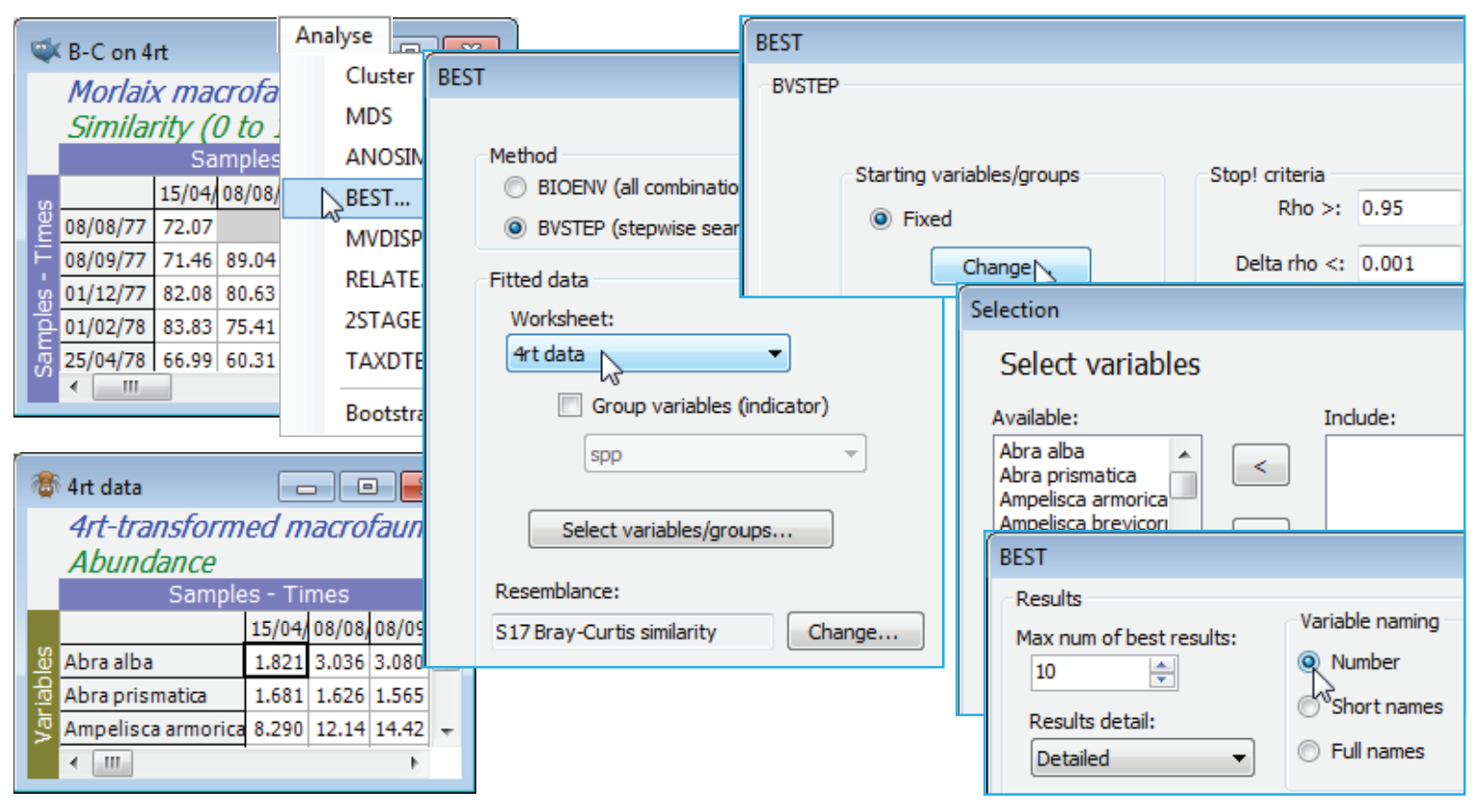
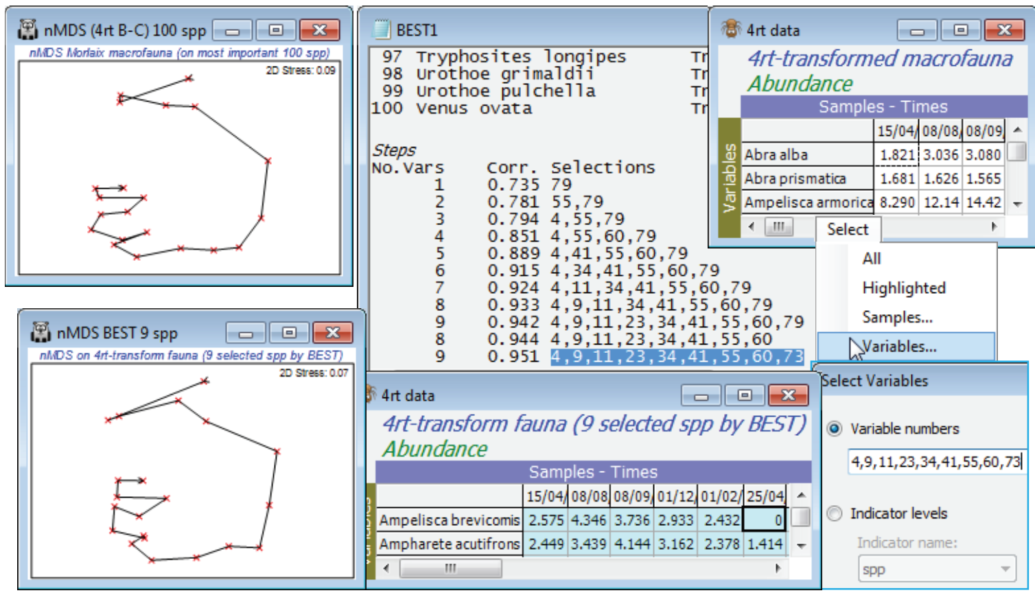
Re-open the Morlaix ws workspace in C:\Examples v7\Morlaix macrofauna from earlier in this section, or since this is all that is needed, just open the data file Morlaix macrofauna abundance into a clear workspace. It consists of 21 sampling times and 251 species. Clarke & Warwick 1998 reasoned that many of these species were sufficiently rare (over half have totals across all samples in single figures) that the problem could be scaled down by removing those – so reduce to the most important 100 (see Section 3). Thus, Select>Variables>(•Use n-most important where n is 100) on Morlaix macrofauna abundance, then fourth-root transform, naming it 4rt data. (A severe transform seems the best choice, otherwise the counts of tens of thousands in a few species will dominate, as can be seen from a shade plot). Generate the nMDS ordination from Bray-Curtis similarities on this reduced, transformed data, calling the resemblance matrix B-C on 4rt. This is the active sheet on entry to Analyse>BEST, which takes the transformed data matrix 4rt data as its secondary sheet and searches for the smallest possible subset of the 125 species that effectively contains (to within $\rho$>0.95) the same among-sample information as B-C on 4rt. It is clear that the full enumeration of possibilities in the (•BIOENV) option would never be possible (2$^{100}$ species combinations!) so the stepwise option of (•BVSTEP) is necessary. Even with the reduction of species numbers, it must be realised that many of these 100 species will be highly inter-correlated, and it is inevitable that many marginally different combinations of species will do an almost equally good job as indicators of the full data set (a point also made in Section 13 about linking biotic and abiotic variables). It is desirable therefore to start the search from several random subsets (perhaps 50), and look at all the output results (Detailed) – if only to appreciate that we are very far from having a single ‘correct’ answer! Nonetheless, it is interesting to see that the detailed MDS based on 100 species can be reproduced almost perfectly by several competing selections of only 8 or 9 species, as follows.
BVStep starting and stopping options
On B-C on 4rt, Analyse>BEST>(Method•BVSTEP) & (Worksheet: 4rt data), taking the defaults for all other entries (Spearman correlations, the suggested Bray-Curtis similarity, all 100 species Available for selection, and the permutation test ignored – a test of $\rho$ = 0 makes no sense in this context and is invalid when the same data are being used in both matrices). On the Next> dialog, for BVSTEP options, take (Starting variables/groups•Fixed), i.e. on the Change button, no species are in the Include category, so the stepwise routine starts from no species and forward steps. An alternative is to Include them all and the routine will then work largely in backward elimination mode, though – as previously mentioned – this tends not to work as well since it can be difficult to drop species that are so sparse that they add or detract nothing. The (Stop! Criteria Rho>: 0.95 & Delta rho<: 0.001) choice ensures that the routine will keep searching until either the improvement in $\rho$ at the next step is <0.001 or the cut-off for acceptable $\rho$ of 0.95 is reached. On the final dialog, take (Results detail: Detailed) & (Variable naming•Number). Use of •Short or •Full names makes it easier to immediately identify the species, but numbers have the advantage that a species list can be copied/pasted from the Results window to the Select>Variables>(•Variable numbers) box, so that the optimal species set can easily be extracted from 4rt data and the similarity and MDS re-run.
BVStep from random starts
Starting the iterative search process from a blank species list is certainly not guaranteed to get you to the best solution (minimum number of species which give $\rho \ge$0.95) – it is easy to get trapped in a local optimum which is not the globally best solution (which can never be known for certain). In fact a marginally better solution, in the sense of involving only 8 species variables, can be found in this case. See this by re-running the routine from different starting places, having first reinstated the full 100-species transformed data matrix 4rt data by Select>All – this is important otherwise you will find yourself searching only through the 9 species! (You may also wish to remove highlights with Edit>Clear Highlight, though this is not important). The first dialog for Analyse>BEST (run on active sheet B-C on 4rt) is the same as previously, but on the BVSTEP dialog take (Starting variables/groups•Random selection)>(Num of trial variables/groups: 6) & (Num of restarts: 25). This starts the stepwise routine from a randomly chosen 6 species from the 100, and (Results detail: Detailed) and (Max num of best results: 25) on the last dialog will allow you to see the alternating backward elimination and forward stepping phases in the Results window. It also permits the final (Best Results) table to display all the solutions obtained – in best to worst order – in the event that they are all different (which they nearly all are in the case below!).
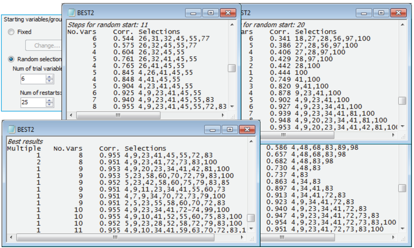
Remember that these are not listed primarily in decreasing order of $\rho$ but in increasing order of the number of species. Only when two sets have the same number of species is the $\rho$ value (which has to be $\ge$0.95 for that solution to be listed at all) taken into account. You will obtain a different set than this (though probably overlapping), since a differing random number seed is used to select the starting species in every new run of the program. Occasionally, the search will end prematurely before 0.95 is reached, even though we know a value of 0.95 exists if we are searching the whole matrix (a value of 1 then exists!) – in that case try using Delta rho<: 0.0001, or even smaller, to try to keep the addition and deletion of species operating, and/or increase the number of restarts. The second-best solution above was found twice (see the Multiple column in the Best Results table) but many more than 25 restarts would probably be needed to be reasonably content that a 7-species solution could not be found. Setting out on an exhaustive search here rather misses the main point, though, that the impact and seasonal structure in the above MDS – which, importantly, is largely ‘signal’ because of the large sample sizes (we are not chasing ‘noise’) – can be displayed in just the same way by a small set of 8 or 9 species. A close look at the near-optimum solutions shows that many of the same species are involved in several of these.
In the further analysis in Fig. 16.3 of CiMC, from the Clarke and Warwick 1998 Oecologia 113 paper (and based on a somewhat larger number of species retained from the original c. 250), BEST is re-run, excluding this first subset of BEST-selected species, but again matching to the B-C on 4rt similarities from the retained set. In the above case, we therefore need to exclude species 4, 9, 23, 41, 45, 55, 72, 83 from the 4rt data matrix before entering it as the (secondary) worksheet to BEST. The quickest way of doing this, as seen earlier, is to copy and paste those 8 numbers to the Select>Variables>(•Variable numbers) box, then Select>All to leave them highlighted, and Edit>Invert Highlighted followed by Select>Highlighted will leave the remainder of the transformed 4rt data matrix selected for this second run of BEST. The matrix then needs to be Tools>Duplicate(d) in order to use the same trick to remove both the first and second species sets selected by BEST, if a third species set is sought. For the Morlaix data, about five entirely separate species peels can be found, all of which essentially reproduce the same multivariate pattern, indicating a high level of structural redundancy in the matrix.
This is the ‘opposite side of the coin’ from the coherent curves analysis we saw for this data in Section 10, where species were grouped into (about 8 or 9) distinct and characteristic sets in terms of their temporal patterns, seasonally and in response to the oil-spill and its aftermath. Each set contains several species which are able to substitute for each other, in the sense that their time patterns are statistically indistinguishable. Conceptually, it should be the combination of the (numerically more dominant) species drawn from each of these sets which tend to make up the above species peels, between them representing the range of temporal responses and therefore capable of recreating the community pattern for the full data set.
Close the Morlaix workspace – it will not be needed again.
Multivariate dispersion MVDISP
One of the few multivariate routines not so far met is Analyse>MVDISP, applied to a resemblance matrix from samples with a simple group structure (i.e. a 1-way layout, or a crossed design that can be turned into a 1-way layout by defining an appropriate combined factor). This gives a description of relative multivariate variability within each of the groups in a single ordination or, to be more precise, in the full-dimensional space of the rank similarity matrix underlying that ordination. (As such it is not a matching of multivariate patterns and doesn’t really belong in this section – but it has to go somewhere!) The concept is again a simple non-parametric one – though rather limited in scope – and described in the Increased Variability section of Chapter 15 in CiMC, so only an example will be given here. Tables of the dispersion sequence of all groups (equation 15.4) and the index of multivariate dispersion (IMD), comparing pairs of groups (equation 15.2), are output to the results window, and these measure differing relative dispersion across groups on the basis of dissimilarity (or any other resemblance measure) within groups – between-group dissimilarities are not used. [If a description retaining the actual similarity scale is required, an alternative – for the special cases of Bray-Curtis and Euclidean distance – might be to run Analyse>SIMPER on the transformed data sheet and look at the headings for the first set of tables, each of which gives the average similarity of all pairs of replicates within that group. More generally – for all other coefficients – the same information about average resemblance within groups is one of the tables output from the PERMANOVA+ add-on routine, PERMDISP, see the Anderson et al 2008 user manual].
The term multivariate dispersion rather than variance is used because the relationship between the univariate variance of the original variables and the dispersion in ‘resemblance space’ (and its low-dimensional ordinations) can be far from linear, depending on the choice of resemblance measure. For example, similarity measures in the quantitative Bray-Curtis family (see earlier this section on comparison of resemblance coefficients) are driven partly by the presence/absence structure of the data, as well as the magnitude of counts from species which are always present, and this inevitably involves a non-linear transformation of original variable scales. Similarly, something as simple as normalisation, used in a Euclidean distance analysis of environmental variables, will remove any direct link between variance on the original measurement scales and dispersion in the multivariate space. Any statement about relative dispersion, therefore, must be contingent on specifying the resemblance measure used. Clarke KR, Somerfield PJ, Chapman MG 2006 J Exp Mar Biol Ecol 330: 55-80, show the radically different conclusions that would be reached, for the Tikus Island reef coral study (met in Section 5), about the dispersion among transects before and after a coral bleaching event, under Chi-squared, Bray-Curtis (standard and zero-adjusted) and Euclidean-based analyses – with the intermediate (zero-adjusted) Bray-Curtis arguably giving the most informative description, in terms of identifying the inter-annual changes in coral community. (This interesting example is also extensively discussed in Chapter 16, CiMC, on resemblance coefficient choice.)
(Mesocosm experiment, Solbergstrand copepods)
The illustration used here is a simple 1-way design of 3 mesocosm treatments: Control (C), Low (L) and High (H) dose of organic enrichment applied to the surface of 12 intact sediment cores, taken from the same location into a mesocosm system, and randomly allocated to the treatments (with 4 replicates in each). Data are from Gee JM et al 1985 J Exp Mar Biol Ecol 91: 247-262, as analysed in a multivariate way by Warwick RM & Clarke KR 1993 “Increased variability as a symptom of stress in marine communities” J Exp Mar Biol Ecol 172: 215-226. Chapter 15, CiMC shows analysis of the resulting meiofaunal communities in the sediment cores (nematodes and copepods) after several weeks’ exposure, but here we open just the copepod data, Solbergstrand copepod counts in C:\Examples v7\Solberg copepods. For square-root transformed data and Bray-Curtis similarities, plot the nMDS and note the apparently much larger dispersion within the High dose treatment (as well as the obvious differences between treatments, which would be tested, validly, by 1-way ANOSIM). This is indicated more reliably, i.e. not in the low-d approximation of an ordination plot, by running Analyse>MVDISP>(Factor name: Treatment) on the resemblance matrix. The dispersion sequence of 0.56, 0.84, 1.60 for L, C, H shows that the average rank dissimilarity is almost three times higher within H than L (comparable dispersions result in a sequence of 1’s), and the pairwise comparisons show that all the lowest dissimilarities (within a group) are in L and all the highest in H (thus IMD = –1 for that pair of treatments). The result, however, is of limited usefulness since an exact permutation test of these dispersion differences is not possible under the non-parametric framework in PRIMER, for much the same reason as interaction tests in a two-way crossed layout are not possible, see the comments at the end of Section 9 and Chapter 6 of CiMC. [No permutation procedure exists under a null hypothesis that the dispersions are the same for each group, but that the ‘locations’ – in so far as they are defined for rank-based dissimilarities – may differ. If the primary interest is in testing for differences in multivariate dispersion of groups, for a given resemblance measure, you should use the (approximate, semi-parametric) permutation test given by the PERMDISP routine in PERMANOVA+ – see the Anderson et al 2008 manual. The parameters defining centroids of each group in the high-d PCO space are estimated and each centroid is moved to the same point, justifying permutation of the samples across groups under the null hypothesis – if location differences have been removed, and the null hypothesis specifies no dispersion differences, then sample labels again become interchangeable.]