15. Biodiversity measures and tests (DIVERSE, TAXDTEST)
- Input/output for diversity; Presentation of diversity information
- Taxonomic distinctness
- Standard indices calculated
- Multivariate analysis of diversities
- (Bermuda macrofauna ); Caswell’s neutral model
- Range of relatedness indices calculated
- Species distance information
- Distances in aggregation worksheets
- Weighting of tree step lengths
- Taxonomic distinctness (European groundfish)
- Box plots & means plots for diversity indices
- Testing taxonomic distinctness against a master list
- TAXDTEST (European groundfish)
- Compute time & limits on path numbers
- Histograms for one sublist size
- Funnels for a range of sublist sizes
- Using taxon frequency in simulations
- ‘Ellipses’ for joint values of ($\Delta^{\scriptscriptstyle +}$, $\Lambda^{\scriptscriptstyle +}$))
Input/output for diversity; Presentation of diversity information
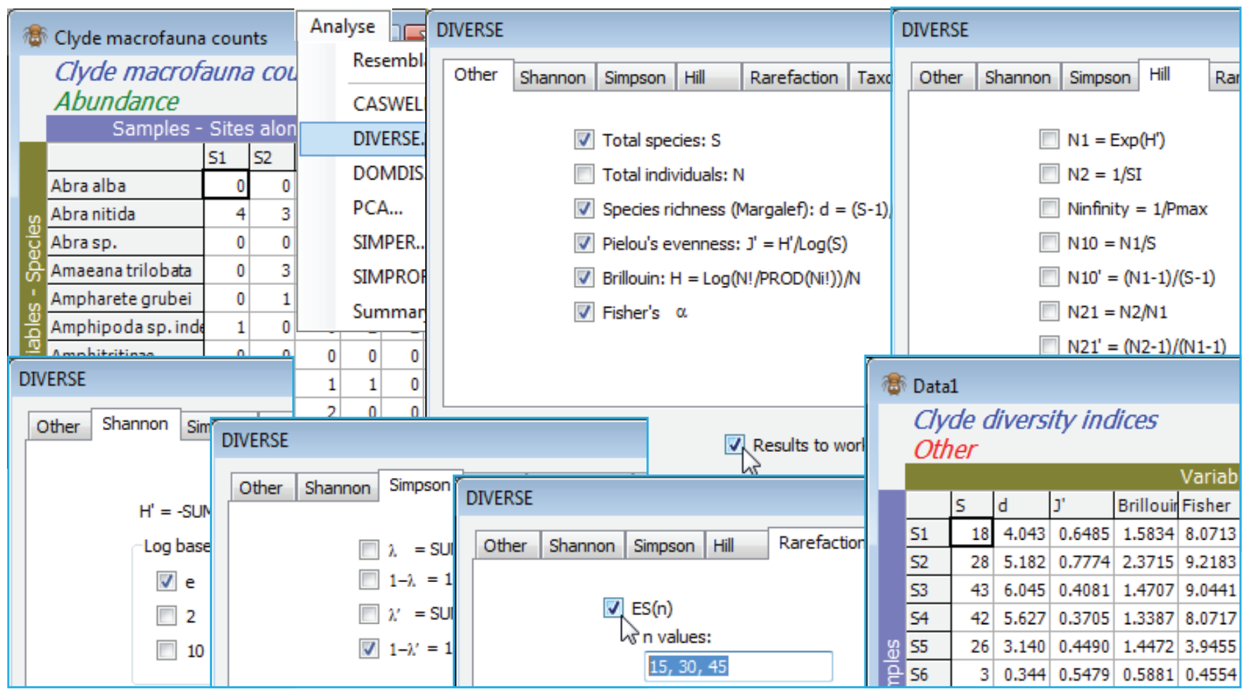
PRIMER computes an extensive set of univariate diversity measures, covering most of the standard indices used in ecology. The active sheet is a data matrix for which the chosen indices are calculated for every sample. The measures are selected by ticking check boxes, so any combination of them can be computed in one run, and the results output either to the results window in a tabular format (which can be copied to the clipboard and pasted directly into Excel) or as a samples-by-variables matrix in a second worksheet. The latter can be saved, as usual, in text or Excel format, for transfer to a standard univariate stats package, but PRIMER 7 can now produce means and confidence interval plots for sets of univariate data, and the PERMANOVA+ add-on can perform permutation-based ANOVA on each variable (univariate being a special case of multivariate).
The facility to send the indices to a new worksheet also allows some interesting possibilities for further presentation, including multivariate analysis. For example, the indices can be superimposed, one at a time, on an MDS plot for the full species assemblage data (treat the diversity matrix like an environmental variables data file) or input the diversity matrix to a multivariate analysis itself (again treat the indices as an environmental array and calculate normalised Euclidean distances between samples for an MDS, or run a PCA). This will show the between-sample relationships obtained from the full range of diversity information extracted, and can be contrasted with the usual ordination exploiting the matching of species identities between samples (which is generally found to be more sensitive, since it exploits more of the available information). A PCA for a large set of diversity indices can also demonstrate how many genuinely different axes of information they have captured (i.e. how many PC axes explain most of the variability), since many standard indices are really just some weighted combination of two features: the total number of species (richness) and the extent to which the total abundance is spread equally amongst the observed species (evenness). An MDS plot of the variables, using (absolute) correlations between indices as the resemblances (an analysis mentioned previously for species, but considered likely to be too high a stress there to be useful) is now viable and shows which measures are essentially equivalent. Such analyses can be an incentive not to proliferate indices by defining yet further variations of the same information.
Taxonomic distinctness
One of the distinctive features of PRIMER is its inclusion of a suite of biodiversity measures based on the relatedness of species within a sample, e.g. the average ‘distance apart’ of any two species or individuals chosen at random from the sample (termed average taxonomic distinctness). This is usually defined from a Linnaean tree (though could be phylogenetic, genetic or functionally-based) and requires availability either of an aggregation file (Section 11) covering all the species in the data matrix, which will be used to compute species distances, or a more direct species resemblance matrix, supplying genetic or functional distances among species. It provides an added dimension of information to that obtainable from the abundance distribution alone: as an average measure its construction makes it independent of the number of species, and it thus has much better statistical sampling properties than richness-related estimators when sampling effort is non-comparable over samples. This should be seen as the major sphere of application: uncontrolled studies over wide spatial or temporal scales, where classic diversity measures can be misleading. Several papers describe the methods, e.g. Clarke KR & Warwick RM 1998, J Appl Ecol 35: 523-531, Clarke KR & Warwick RM 2001, Mar Ecol Prog Ser 216: 265-278 and Warwick RM & Clarke KR 2001, Oceanog Mar Biol Ann Rev 39: 207-231. A detailed exposition is also given in Chapter 17, CiMC.
In just the same way as for the classic indices, PRIMER can calculate a range of such taxonomic-related measures (including the PD of Faith DP 1992, Biol Conserv 61: 1-10), through check boxes on the Analyse>DIVERSE menu. These can be separated into quantitative indices (e.g. $\Delta$, $\Delta ^\ast$) and those which depend only on a species list (indicated by a superscript +). The latter are divided into average measures (e.g. $\Delta ^+$, $ \Lambda ^+$) which have the property of independence of sampling effort (in their mean values), and total measures (e.g. S$\Delta ^+$, S$ \Phi ^+$) which are alternative definitions of the taxonomic richness, combining the number of species with relatedness information. For two of the presence/ absence measures, a hypothesis testing structure can be erected to compare a location’s observed average taxonomic distinctness (AvTD, $\Delta ^+$) and variation in taxonomic distinctness (VarTD, $ \Lambda ^+$) with that ‘expected’ from a regional master list, assuming assembly rules for the species set which are independent of their taxonomic inter-relation. This is run by Analyse>TAXDTEST, when the active window is either an aggregation file or a variable (dis)similarity matrix.
Standard indices calculated
The range of indices available is illustrated with the macrobenthic data Clyde macrofauna counts from the Clyde sludge dump-ground study, directory C:\Examples v7\Clyde macrofauna, last seen in Section 14. Analyses so far have used only the abiotic and biomass matrices, and the existing workspace Clyde ws may have become cluttered, so open Clyde macrofauna counts into a new workspace, and save it as Clyde ws2. Without pre-treatment, take Analyse>DIVERSE>(✓Results to worksheet). Look at the options on the first 5 tabs, taking only ✓S, ✓d, ✓J$^\prime$, ✓H, ✓$\alpha$, ✓H$^\prime$ (log base e), ✓1 – $\lambda^\prime$, ✓ES(n) with n values: 15, 30, 45 (there is no special significance to the index grouping under tabs, except that the last two tabs deal with taxonomic-relatedness measures, seen later). The abundance of the ith species is denoted by N$_i$ (i = 1, 2, .., S) and, as a ratio of their sum (N), this is denoted P$_i$ (i = 1, 2, .., S). The first 5 tabs (where ✓ denotes the default selections) are:
Other
✓Total species: $S$
✓Total individuals: $N$
✓Species richness (Margalef): $d = (S – 1)/\log_e N$
✓Pielou’s evenness: $J^\prime = H^\prime / \log_e S$
Brillouin: $H = N^{-1} \log_e \{ N! / (N_1!N_2!…N_S! ) \} $
Fisher’s $\alpha$ statistic
Shannon
✓$H^\prime = – \sum P_i \log(P_i)$, where the logs are to the base e
$H^\prime$ as above but for logs to the base 2
$H^\prime$ as above but for logs to the base 10
Simpson
$\lambda= \sum P_i^2$
$1 - \lambda= 1- (\sum P_i^2)$
$\lambda^\prime= \{ \sum_i N_i (N_i–1)\} / \{N(N–1) \}$
✓$1-\lambda^\prime= 1- \{ \sum_i N_i (N_i–1)\} / \{N(N–1) \}$
Hill numbers
$N1 = \exp (H^\prime)$
$N2 = 1/ \sum P_i^2$
$N_ \infty = 1/ \max_i \{P_i\}$
$N_{10} = N1/S$
${N_{10}}^\prime = (N1–1)/(S–1)$
$N_{21} = N2/N1$
${N_{21}}^\prime = (N2-1)/(N1-1)$
Rarefaction (Sanders/Hurlbert)
$ES_n$, the ‘expected’ number of species from $n$ individuals ($n \le N$)
Multivariate analysis of diversities
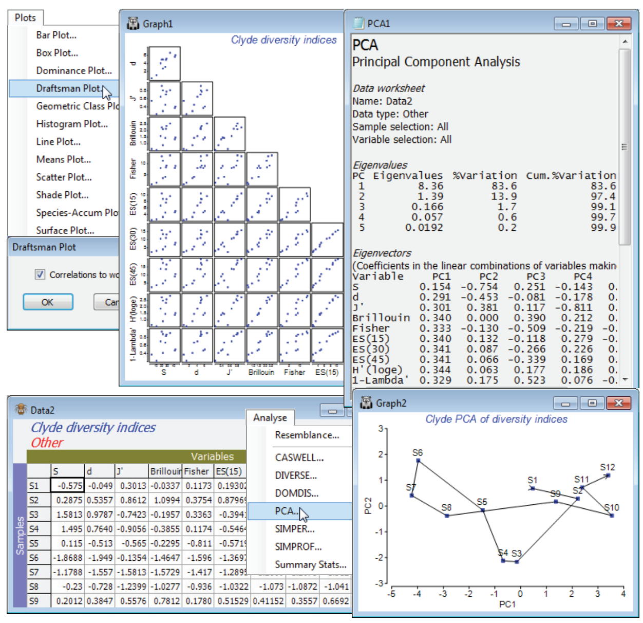
For the diversity (variables) by samples matrix, Data1, Plots>Draftsman Plot>(✓Correlations to worksheet) shows that none of the indices is badly behaved, i.e. skewed, dominated by outliers, strongly curvilinear relationships etc., so no transforms seem called for. [To get the plot below, you might find it helpful to increase the symbol size on the Samp. labels & symbols tab, and on the X & Y axis tabs increase the title font sizes, unchecking (✓Limit size)]. Data1 needs Pre-treatment>Normalise Variables, however, before entry to Analyse>PCA since the indices are on different scales. On the configuration plot from PCA, turn off (✓Overlay vectors) on Special>Overlays and instead (✓Overlay trajectory) of the transect Site#. Site 6 is the dumpground centre, with Sites 1 and 12 at the extremities of the transect, and this combined set of diversity indices clearly displays the strong, simple gradient of effect, in a rather similar way to the full multivariate analysis of the original species data (you might like to carry out the latter, with a fairly severe transformation and Bray-Curtis similarities). The agreement is a consequence of the severity of the impact. The meta-analysis of Chapter 15 of CiMC shows this to be the most severe of the contaminant studies looked at there, but Chapter 14 also shows that such agreement is untypical, diversity measures being less likely to detect biological change for more intermediate-level disturbances. The PCA results (the eigenvalues) also make it clear that rather little is to be gained by calculating ten diversity indices instead of two or three: over 83% of the total variation in the 10 indices is accounted for by the first PC, and 97% (i.e. all of it, in effect) by the first two PC’s. The coefficients (eigenvectors) show that the simple left to right gradient in the main axis (PC1) of the PCA is a roughly equally weighted combination of all measures (evenness + richness), both increasing away from the dumpground, whereas the second axis strongly contrasts the two main diversity components: PC2 is effectively (evenness – richness). This simplicity should not be a surprise, given the high correlations between indices evident from the draftsman plot, and from the correlation matrix Resem1 created with it.
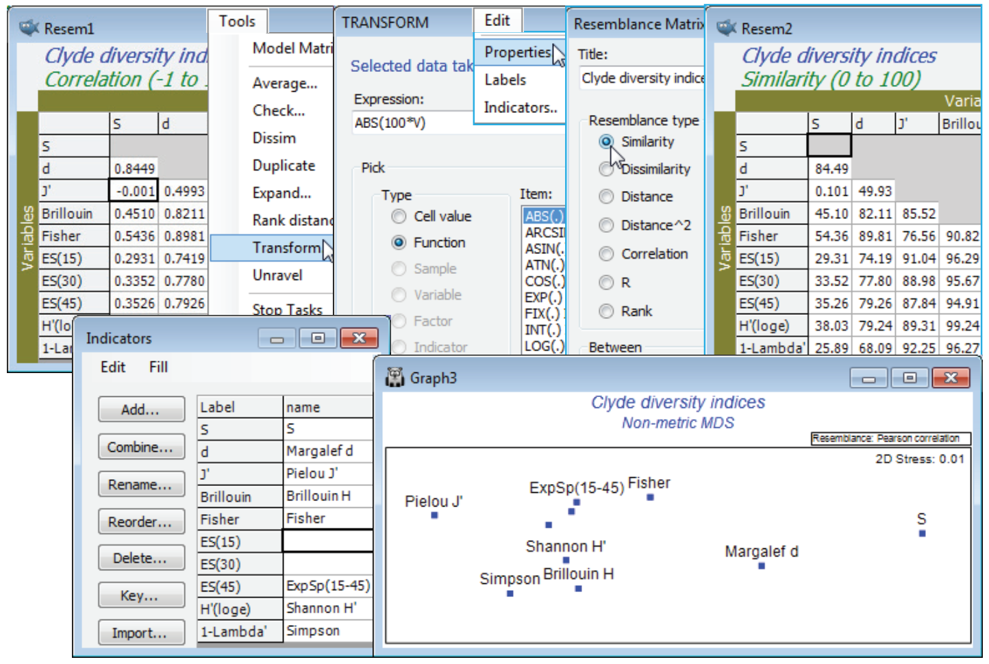
A final, revealing plot can be produced from Resem1, by ordinating the variables. Technically, it first needs transforming before it can be considered a similarity matrix: there is a small, negative correlation between S and J$^{\hspace{2pt} \prime}$. It is effectively zero here, but other situations might produce large negative correlations, e.g. between equitability and dominance measures, and they should also imply similarity (of variables). Tools>Transform>(Expression: 100*ABS(V)) on Resem1 will achieve the conversion to a similarity matrix (and you could change its type on Edit>Properties). Then Analyse>MDS>Non-metric MDS (nMDS) generates the ordination plot for the variables shown below, in which the relative distances apart of the indices exactly reflects the rank order of their pairwise correlations (note that the MDS stress is effectively zero). The plot is largely linear, the extremities corresponding to pure richness (S) and evenness (J$^{\hspace{2pt} \prime}$), with other measures being a mix of these two components. The points have been more descriptively labelled using Var. labels & symbols>(Labels✓By indicator)>Edit, which is equivalent to Edit>Indicators on the Resem1 sheet, then Add an indicator: name. The boundary of the nMDS plot has also been appropriately reshaped for this linear plot, with Special>Main>(Plot type•2D>Aspect ratio: 3). Values of n = 15, 30 and 45 were chosen for the rarefaction indices ES(n) because larger values are not permissible, the site with lowest abundance having only 46 individuals. (To see this Analyse>Summary Stats>(For•Samples)>(✓Sum) on Clyde macrofauna counts, or just ask for ✓N in Analyse>DIVERSE). The fact that the expected species numbers ES(n) are clearly considerably closer to being evenness measures than the richness indices that their name implies (correlations of about 0.9 with J$^{\hspace{2pt} \prime}$ and 0.98 with H$^{\hspace{2pt} \prime}$, compared with about 0.3 with S) results from the lack of ecological realism in their underpinning model. This assumes that individuals arrive randomly and independently into the sample, and hence the process can be reversed in rarefaction, by randomly excluding them. This does not correspond to the reality of a clumped spatial distribution seen for many species (as seen in Dispersion Weighting, Section 4). Resave the workspace Clyde ws2 for later use, and close it.
(Bermuda macrofauna ); Caswell’s neutral model
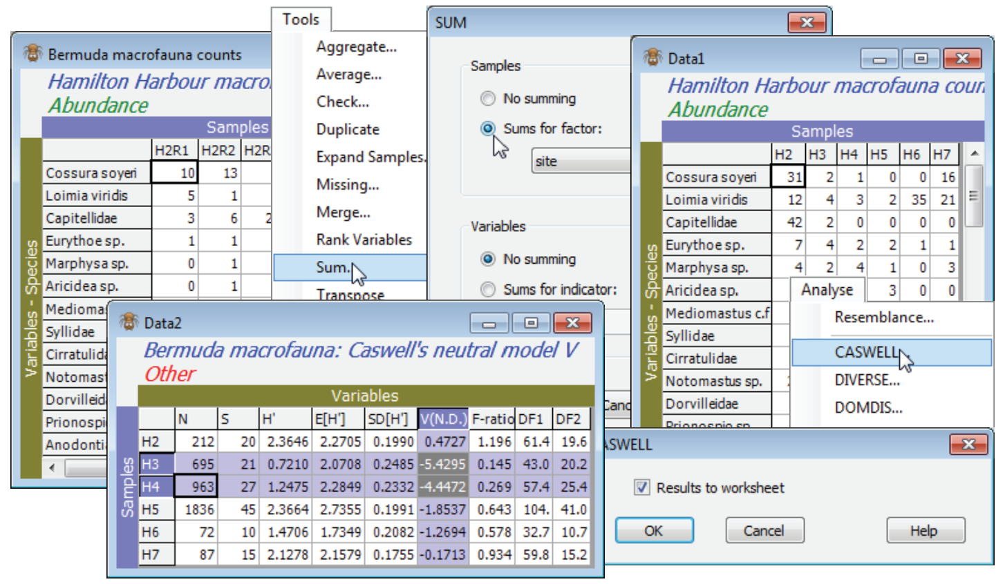
Soft-sediment macrofaunal assemblages (along with meiofauna and biomarker suites) were studied at 6 sites in Hamilton Harbour, Bermuda (labelled H2, H3, H4, H5, H6, H7) during an international IOC workshop on the effects of pollutants in sub-tropical waters (Addison RF & Clarke KR, eds 1990, J Exp Mar Biol Ecol 138). There were 4 replicates at each site, giving a data matrix of 24 samples from 64 species, in the data file Bermuda macrofauna counts in directory C:\Examples v7\ Bermuda benthos. These data will be used to illustrate computation of another diversity index, not now widely used (the validity of its assumptions being questionable for most assemblages) but which has been available in PRIMER from early versions and therefore retained for consistency.
Analyse>CASWELL generates V statistics for the Caswell neutral model, and is discussed in Chapter 8 of CiMC. It is essentially a comparison of Shannon diversity H$^{\hspace{2pt} \prime}$ with the value it would be expected to take, conditional on the observed number of species S and individuals N, under some simple model assembly rules for the community, which are ecologically neutral, in the sense defined by Caswell H 1976, Ecol Monogr 46: 327-354. The normalised form of H$^{\hspace{2pt} \prime}$ (subtract the modelled mean and divide by the modelled standard deviation) is the V statistic, positive values of V implying greater diversity than neutrality and negative values lesser. (There is an F test of its departure from V = 0, though this is not very convincing because it also depends on the neutral model assumptions, which are unrealistic for typical assemblages). The algorithm implemented here is due to Goldman N & Lambshead PJD 1989, Mar Ecol Prog Ser 50: 255-261.
Recreate the Caswell example in Chapter 8 of CiMC, for the Bermuda macrofauna counts by firstly summing across the replicates, to increase the sample size, with Tools>Sum>(Samples•Sums for factor: site) & (Variables•No summing). This is justified because there is equal replication at each site – Tools>Average would not be appropriate for a Caswell calculation because the entries are no longer real (integer) counts. Note that V could alternatively be calculated for each replicate, as for the diversity measures above, and this would allow standard means and confidence intervals based on variance estimates from replication, rather than the (less robust) internal variance estimate from the neutral model. On the summed Data1 take Analyse>CASWELL>(✓Results to worksheet), and the V values for each site (and the accompanying test calculations) are found in the resulting Data2 sheet, which can be manipulated, saved etc. as with any other data matrix. Sites H3 and H4 are seen to have H$^{\hspace{2pt} \prime}$ well below expectation under the neutral model (V statistics of -5.4, -4.5 respectively). Close the workspace – it will not be needed again.
Range of relatedness indices calculated
In order to obtain a diversity measure which steps outside the species abundance distribution, and which could therefore potentially strike out along a different axis to the linear richness-evenness combinations shown in the MDS of the mechanistic correlations among standard diversity indices, it would be helpful to introduce further attributes of the assemblage composition. One possibility is to combine biomass and abundance data, as in ABC curves (Section 16), but another – which we shall turn to now – is to introduce information on the relatedness of the species in each sample, as discussed at the start of this section. These indices are accessed through the final two tabs of the dialog box from Analyse>DIVERSE, namely Taxdisc and Phylogenetic. The nomenclature comes from the original papers on these topics (Warwick and Clarke’s taxonomic diversity and taxonomic distinctness indices, and Faith’s phylogenetic diversity), and does not imply that either set of indices is more appropriate to taxonomic or phylogenetic hierarchies. Other hierarchies (e.g. genetic, functional) could be equally appropriate and PRIMER does not now even need a hierarchy to compute the taxonomic distinctness measures – a distance among species matrix will suffice.
Taxonomic distinctness
Quantitative:
Taxonomic diversity: $\Delta$
Taxonomic distinctness: $\Delta^\ast$
Presence/absence:
Average taxonomic distinctness (AvTD): $\Delta^+$
Total taxonomic distinctness (TTD): $S\Delta^+$
Variation in taxonomic distinctness (VarTD): $\Lambda^+$
Phylogenetic diversity
Presence/absence:
Average phylogenetic diversity (AvPD): $\Phi^+$
(Total) phylogenetic diversity: $S \Phi^+$ (Faith’s ‘PD’)
Species distance information
For the first set of measures (on the Taxdisc tab), the Taxonomy button gives a choice of whether the distances among species (or whatever the variables represent) are provided by a tree structure (•Taxonomy) or a direct distance matrix among species (•Resemblance). The latter then requires a Variable resemblance matrix to be specified (perhaps one calculated among species on the basis of their traits, if this is to be a functional rather than taxonomic-based distinctness index). The former requires a Variable information sheet – usually an aggregation file of the type seen near the start of Section 11 – which needs to be in the workspace before Analyse>DIVERSE is run (if only one such file has been read in, it will be the default). This is a look-up table which gives a taxonomic (or other) tree of all species, allowing the routine to calculate species distances internally (these are not actually output but could be so, if needed, by Analyse>Similarity when the active window is the aggregation worksheet, as seen in Section 5). For the second set of measures (the Phylogenetic tab in the DIVERSE dialog), the Taxonomy button offers only the option to input a Variable info. worksheet because the PD measures ($\Phi^+$ and $S \Phi^+$) can only be computed from a species tree and not from a triangular matrix of between-species distances.
Distances in aggregation worksheets
Such tree structures (e.g. taxonomies) are one of a distinct worksheet type, Variable Information, slightly expanded in PRIMER 7 from the aggregation file format of PRIMER 6, but still with an *.agg extension when saved as PRIMER 7 binary format – they can also be input or output in *.xls or *.xlsx Excel format. The aggregation matrix could simply be a tree constructed for just those species in the current data matrix or it could be a wider and more comprehensive master list for those faunal groups. The species (or other variable) labels used in the data worksheet must find an exact match in the labels of the aggregation sheet (or, if working from a higher taxonomic level in the aggregation matrix, e.g. genus, used as the variable names for the data sheet, then this must be specified in Current level of sample data). The species do not need to occur in the same order in the both sheets because of PRIMER’s use of strict label matching. See Section 11 for information on checking aggregation arrays for inconsistency – potential mis-spellings – with Tools>Check.

There are also options under the Taxonomy (Data) dialog to use only part of the taxonomic tree. For example, (Use links)>(From level: Genus) would start from genus level – in effect treating all species in the same genus as the same taxon – which is not often a requirement but could be useful if the identifications are very patchy to the species level, but reliable to genus. Similarly, the tree could be compressed at the top level so that, for example, no greater distance is assumed between two species in different classes than for two species in different orders but the same class – that would be achieved by specifying (Use links)>(To level: Order).
Weighting of tree step lengths
The other box in this Taxonomy (data) dialog can be used to alter the weights given to the various branch lengths in the tree (and includes the previous compression at the top or bottom of the tree as a special case, with those step lengths set to zero). By taking (Weights•User specified)>Weights, the default lengths are displayed: equal steps are assumed, and any values placed here will always be standardised, subsequently (and automatically), so that the longest path in the tree is set to 100. Thus a change to step lengths of 2 for all categories would not alter the values of any of indices, but a change to decreasing step lengths of 6 (species to genus), 5 (genus to family), 4 (family to order) etc. could be worth exploring because it would put relatively more weight on the shorter branch lengths between species (of which there are fewer) rather than leaving much of the emphasis on the longer branch lengths (because there are many). One logical basis for altering the step lengths from their default would be to make them depend on the decrease in the number of taxa in the master list when making that step – the smaller the decrease in the number of taxa, the shorter the step length. This has the merit of consistency if, for example, an arbitrary taxonomic level (e.g. subfamily) is interpolated but not used (i.e. there are as many subfamilies as families in the master list). The set of distinctness indices would then remain unchanged. The detail is given in Clarke KR & Warwick RM 1999, Mar Ecol Prog Ser 184: 21-29, and their weighting scheme can be implemented here by taking (Weights•Taxon richness) in the Taxonomy (Data) dialog box.
Taxonomic distinctness (European groundfish)
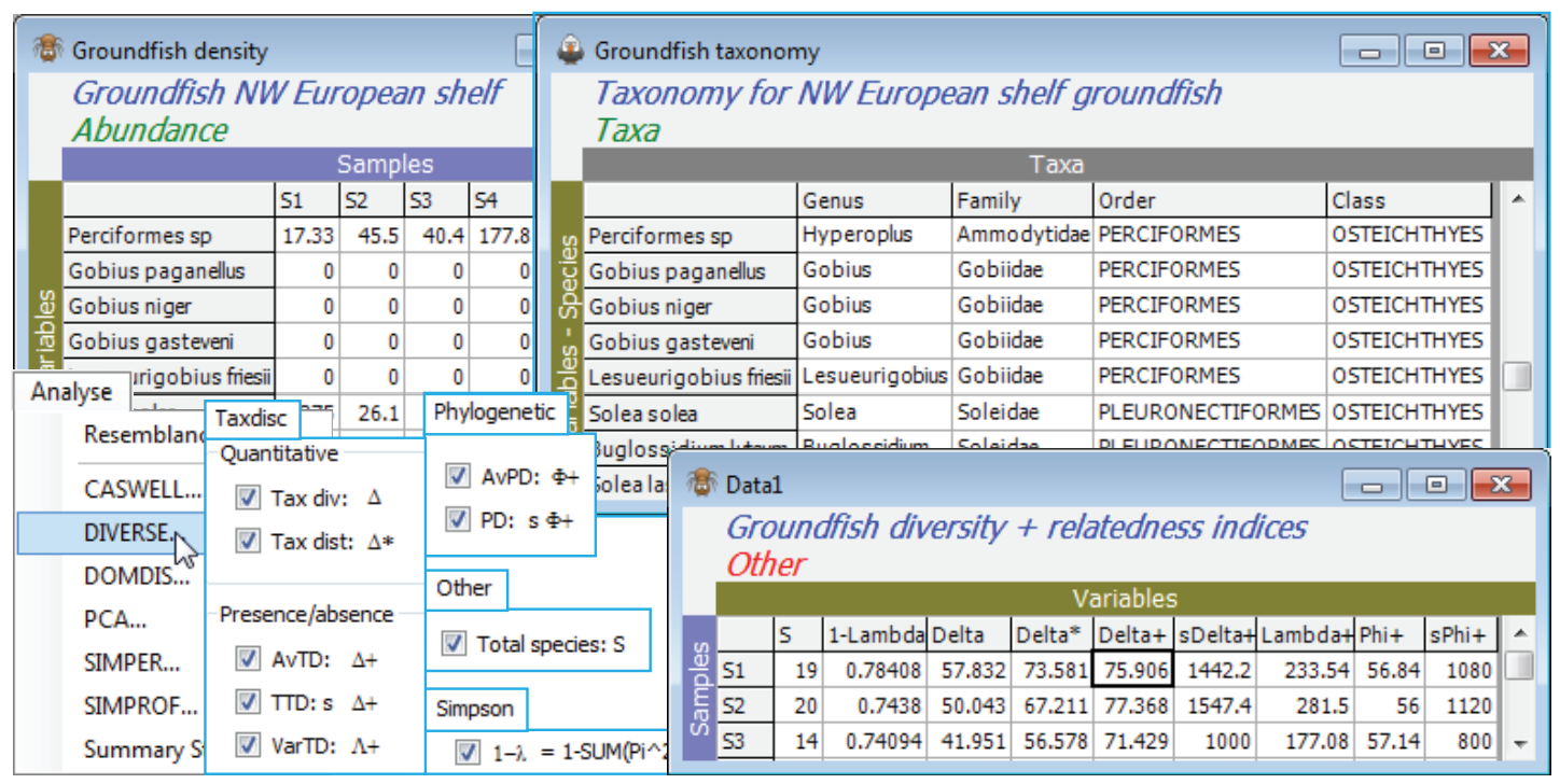
The aggregation matrix for the NW European beam-trawl survey data on groundfish assemblages (93 species in 277 samples, from 9 sea areas) was last seen in Section 11, where it was checked for consistency. However, the workspace is now rather cluttered so open a new one in C:\Examples v7 \Europe groundfish, containing data Groundfish density and Groundfish taxonomy, and save it as Groundfish ws2. Here, data and aggregation matrices have the same full set of species, in the same order. With Groundfish density as active sheet, run Analyse>DIVERSE and on the Taxdisc and Phylogenetic tabs, check (✓) all the quantitative and presence/absence options: $\Delta$ (= delta), $\Delta^\ast$, $\Delta^{\scriptscriptstyle +}$, $S \Delta^{\scriptscriptstyle +}$, $\Lambda^{\scriptscriptstyle +}$ (= lambda+), $\Phi^{\scriptscriptstyle +}$ (= phi+) and $S \Phi^{\scriptscriptstyle +}$, taking also (✓Results to worksheet). Under Taxonomy>(Type•Taxonomy) take all the defaults: (Variable info. worksheet: Groundfish taxonomy) & (Current level of sample data: Species) & (Use links>(From level: Species) & (To level: Class)) & (Weights•User specified), with the Weights left on their values of step lengths of 1 between all levels. Take also the number of species ($S$) and Simpson evenness $1-\lambda$, from the Other tab. Look at the correlation between these indices by Plots>Draftsman Plot. (To obtain the plot overleaf, the axis scales have been switched off by unchecking (✓Show scales) from Graph>Special).
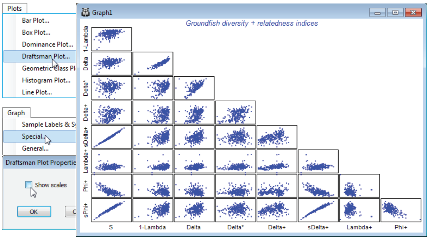
In the draftsman plot, note particularly the first column of plots, which set each index against the number of species, $S$. These bear out the general observations of Clarke KR & Warwick RM 2001, Mar Ecol Prog Ser 216: 265-278, and Chapter 17 of the CiMC manual, that:
- a) total phylogenetic diversity PD ($S \Phi^{\scriptscriptstyle +}$) and total taxonomic distinctness TTD ($S \Delta^{\scriptscriptstyle +}$) are dominated by $S$ (which will be strongly influenced by the differing sampling effort for the 277 rectangles);
- b) an attempt to correct for this by using average PD ($\Phi^{\scriptscriptstyle +}$) is unsuccessful, there still being a strong correlation with $S$ (negative now), but it is successful for average taxonomic distinctness AvTD ($\Delta^{\scriptscriptstyle +}$) and variation in taxonomic distinctness VarTD ($\Lambda^{\scriptscriptstyle +}$), Clarke & Warwick 2001 showing that (mechanistic) independence of $\Delta^{\scriptscriptstyle +}$ and $\Lambda^{\scriptscriptstyle +}$ from $S$ is to be expected on theoretical grounds;
- c) quantitative taxonomic diversity ($\Delta$) retains a strong element of the evenness component from the species abundance distribution, i.e. is strongly correlated with Simpson’s 1–$\lambda$. In fact, $\Delta$ is a compounding of Simpson’s $1-\lambda$ and a pure relatedness index, thus quantitative taxonomic distinctness $\Delta^\ast = \Delta/(1–\lambda$) more nearly represents pure relatedness, and is seen to be much less positively correlated with evenness (here as Simpson $1-\lambda$ but the same is true for Pielou’s $J^\prime$, or even Shannon $H^\prime$ – which is largely an evenness measure, with a small component of $S$);
- d) the quantitative ($\Delta^\ast$) and pres/abs ($\Delta^{\scriptscriptstyle +}$) forms of AvTD, though positively correlated ($\approx 0.5$), are not highly so, suggesting (as other evidence does) that they capture somewhat different aspects of relatedness and are both worth examining when quantitative data exists;
- e) because of their use of the taxonomic tree structure, the taxonomic distinctness measures capture an axis of variation in the samples not reflected by the standard diversity measures (this can be seen by repeating the PCA, and the MDS variables ordination, near the start of this section, for the above relatedness indices together with the classic measures $S$, $d$, $J^\prime$, $H$, $\alpha$, $H^\prime$ and $1-\lambda^\prime$).
Box plots & means plots for diversity indices
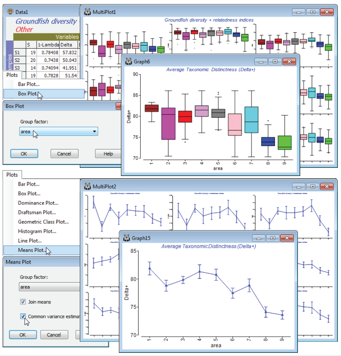
The sheet Data1 of this suite of diversity indices for each of the 277 samples, split into 9 sea areas (factor area), could now be input to two new multi-plot routines in PRIMER 7, namely standard univariate box plots and means plots, treating the sea areas (1: Bristol Channel, …, 9: E Central North Sea; see map Fig. 17.10 in CiMC) as a group structure, with an average of about 30 replicate sample boxes (quarter degree rectangles) within each sea area. Taking Plots>Box Plot>(Group factor: area) on Data1 gives 9 separate box plots, Graph2 to Graph10, one for each diversity index in the above set, each with 9 ‘box and whiskers’ constructions, one for each area. These are placed into a multi-plot, MultiPlot1, and are intended as ‘quick look’ plots, with limited flexibility for manipulation (individual plots restricted to choice of axis scales, title content and text sizes). For Data1 again, Plots>Means Plot>(Group factor: area) & (✓Join means) & (✓Common variance estimate) gives a similar set of 9 plots within MultiPlot2, each of observed means and confidence intervals for the true mean of that particular diversity index for each of the 9 areas. There is choice of separate variance estimates for each area, or a common variance estimate (as from the ANOVA residual mean square). Interval widths for means vary here because areas have differing replication.
Testing taxonomic distinctness against a master list
Wide-ranging biogeographic studies, and particularly historic data, are often restricted to simple species lists. Even where quantitative information exists, it is rarely from sampling protocols that have been standardised with respect to sampling effort over the whole data. Where sampling is so exhaustive that the asymptote of the species-area curve is approached, then it may be valid to compare diversity status by the length of these lists (species richness $S$), but this is not often the case (in marine science, certainly). As is well known, $S$ is heavily sampling effort dependent so, if sampling effort is variable and unknown, any valid statements about richness appear problematic. However, the two relatedness measures discussed earlier, average taxonomic distinctness (AvTD, $\Delta^{\scriptscriptstyle +}$) and variation in taxonomic distinctness (VarTD, $\Lambda^{\scriptscriptstyle +}$), can not only be calculated from simple species lists, with the added knowledge of their Linnaean (or other) classification, but also possess a robustness to the varying number of species $S$ in the lists. To be more precise, in different-sized sublists generated by random sampling from a larger list (simulating the action of sampling with variable effort) their mean values are unchanged. This suggests that it is valid to compare $\Delta^{\scriptscriptstyle +}$ (or $\Lambda^{\scriptscriptstyle +}$) over historic time or biogeographic space scales, under conditions of variable sampling effort. (Note that the indices are average not total measures, and orthogonal to species richness – along a third PC diversity axis, would be one way of thinking of it – and therefore an addition to $S$, rather than a substitute for it, in cases where sampling effort is controlled and $S$ can be validly compared.)
Furthermore, a test can be constructed for the null hypothesis that a species list from one locality (or time) has the same taxonomic distinctness structure as a ‘master’ list (e.g. of all species in that biogeographic region) from which it is drawn. This is again by simple randomisation: given there are s species observed in a particular sample, make repeated drawings at random of s species from the master list and compute $\Delta^{\scriptscriptstyle +}$ for each drawing, building up a histogram and a 95% probability range of values of $\Delta^{\scriptscriptstyle +}$ expected under the null hypothesis, with which the true $\Delta^{\scriptscriptstyle +}$ can be compared. Values below the lower probability limit suggest a biodiversity that is ‘below expectation’. This can be carried out for a range of sublist sizes and the limits plotted against s, to give a 95% funnel plot of expected values (the funnel arises from uncertainty being greater for smaller sublists). This can be repeated for VarTD ($\Lambda^{\scriptscriptstyle +}$), giving a second set of histograms and funnel. Together, the true $\Delta^{\scriptscriptstyle +}$ and $\Lambda^{\scriptscriptstyle +}$, and the simulated values obtained by drawing their number of species from the master list, can be plotted on a single (x,y) scatter plot. Probability regions (‘egg-shaped’ contours, called ellipse plots since they are back-transformed ellipses) covering 95% of the simulated values can be drawn for a range of sample sizes, and the true ($\Delta^{\scriptscriptstyle +}$, $\Lambda^{\scriptscriptstyle +}$) compared with their appropriate contour.
TAXDTEST (European groundfish)
Further theoretical details and discussion can be found in Chapter 17 of CiMC, which also presents analyses for the Europe groundfish data, whose workspace Groundfish ws2 should still be open. These taxonomic distinctness tests (on presence/absence data only) are accessed by Analyse>TAXDTEST when the active window is either a variable information sheet (an aggregation file) or a variable resemblance matrix. These determine the master list (Master taxonomy on the TAXDTEST dialog box) from which random subsets of species will be drawn, in order to construct the probability histogram, funnel or ellipse plots. It is also the default aggregation sheet used in calculating the observed $\Delta^{\scriptscriptstyle +}$ and $\Lambda^{\scriptscriptstyle +}$ for any specific set of samples, to superimpose as points on the simulated funnels or ellipses (Sample data✓Use Sample data>Taxonomy•Use master). However, with (Taxonomy•Specify different>Taxonomy), a different aggregation sheet could be supplied, for the sample data calculation only. This would normally be quite unnecessary because the species relatedness needed for any particular sample can be drawn from the master taxonomy: as noted earlier, there is no necessity for the sample data matrix to contain all the same species in the same order as the aggregation (or variable resemblance) sheet – it is just necessary that all the species are found in the master list. However, it could be valid to place data from a region (or geological time), with its own aggregation information, on an expected funnel from an entirely different region (or time), with a different master list, so this option is catered for. If based on a variable information sheet (aggregation file), Taxonomy buttons will give the dialog seen earlier, allowing compression of the taxonomic tree and path step lengths which can be altered from equal weighting.
Compute time & limits on path numbers
A new option in PRIMER 7 recognises that computation time can become an issue for particular relatedness analyses when the master list is extremely large - as could happen if, for example, the world list of fish species, or the entire marine species directory of European waters is input as the master list (a species list of 10,000 has 100 million path lengths between all pairs of species). But it is not necessary to calculate all of these to know the true AvTD $\Delta^{\scriptscriptstyle +}$ of the master list, for example – we can again exploit the unbiasedness of random samples to get all the accuracy we need without complete computation, and this option is taken with (✓Limit no. paths)>(Max paths: 9999), say. This option was also provided for distinctness estimates in the DIVERSE routine but may be less necessary there and is inappropriate, so should be avoided, for the quantitative $\Delta$, $\Delta ^\ast$ calculations. Path limitations are not the default and are best saved for use only when essential to obtain results.
Histograms for one sublist size
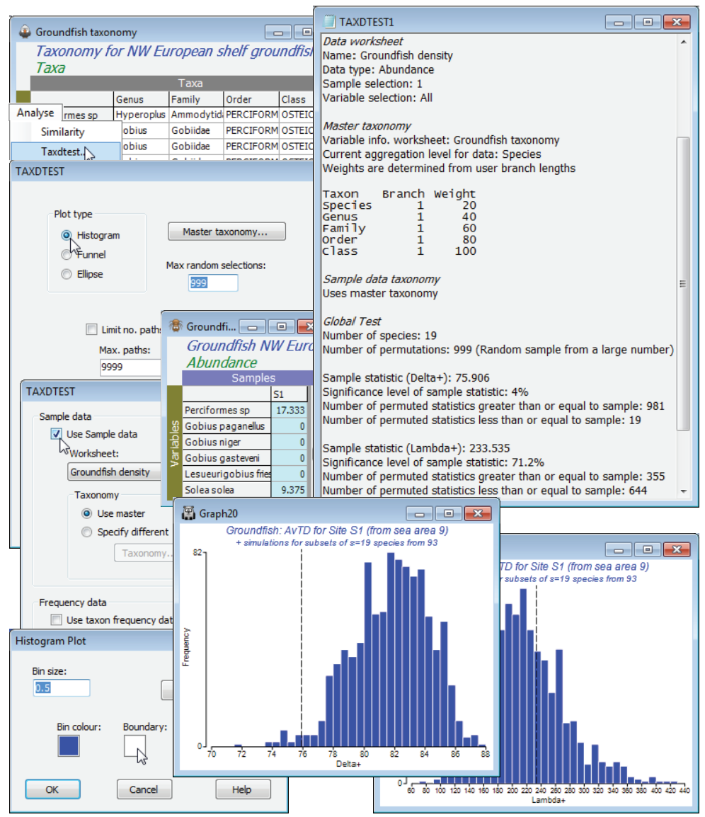
For an example, take the first of the 277 groundfish samples, the 0.25$^\circ$ rectangle S1. Highlight and select just this column from Groundfish density, with Select>Highlighted (this is a quantitative matrix not presence/absence, but TAXDTEST will automatically convert it to P/A data – as does DIVERSE when computing $\Delta^{\scriptscriptstyle +}$, $\Lambda^{\scriptscriptstyle +}$ etc.). With the Groundfish taxonomy sheet as active window, run Analyse>TAXDTEST>(Plot type•Histogram) & (Max random selections: 999), with defaults for the Master taxonomy button and, on the next screen, check (Sample data✓Use Sample data)> (Worksheet: Groundfish density)>(Taxonomy• Use master). Leave the (Frequency data) section for now – it will be demonstrated later. The routine counts S = 19 species in the supplied sample data column so produces 1000 random draws of 19 species from the master list, Groundfish taxonomy. It then calculates $\Delta^{\scriptscriptstyle +}$ and $\Lambda^{\scriptscriptstyle +}$ for each random draw and puts the values into a histogram for each index. The real values of $\Delta^{\scriptscriptstyle +}$ and $\Lambda^{\scriptscriptstyle +}$ for that data column are shown by a dashed line, as usual, and the significance levels (here, for a two-sided test) are given in the results window. In this case, only 19 of the 999 random draws gave $\Delta^{\scriptscriptstyle +}$ values less than or equal to the real $\Delta^{\scriptscriptstyle +}$. The probability of this under the null hypothesis (that species at that S1 location are representative of the full taxonomic spread in the master list of 93, so retain the overall biodiversity) is $\le$(19+1)/(999+1) = 0.02, i.e. a significance level of $\le$2% on a one-sided test. It is arguable here that the test should be one-sided, and that the only departure of interest from the null is one of decreasing taxonomic distinctness – perhaps through extensive beam-trawling differentially affecting groups of groundfish higher taxa with particular life-history characteristics. There may, however, be situations in which we would like also to be able to detect increases in $\Delta^{\scriptscriptstyle +}$, and it is certainly true for $\Lambda^{\scriptscriptstyle +}$ that plausible alternatives to the null hypothesis could be two-sided. So PRIMER quotes two-sided significance levels in both cases (thus a significance of 4.0% for $\Delta^{\scriptscriptstyle +}$) – a one-sided test would simply halve the quoted values. Also remember that each run will give slightly different results because of different random draws, and in borderline cases you might want to increase the number of random draws, e.g. to 9999.
The histograms are displayed in a multiplot, with just the two component plots. The usual display options are accessed through the Graph>General menu, to change overall font size, titles etc., and Graph>Special has here allowed the bin size to be increased for a smoother histogram, and can allow colour change of the histogram bars and boundary (the latter from black to white here).
If you submit several columns of data by mistake at this stage, the error message Only one sample must be selected for histogram will result. If you wish to generate histograms of expected $\Delta^{\scriptscriptstyle +}$ (or $\Lambda^{\scriptscriptstyle +}$) values from the master list, for a fixed sample size (e.g. S = 20), without referring to a specific data sample, then uncheck (✓Use Sample data) in the TAXDTEST dialog. You will then be asked to supply that size, e.g. Histogram>S value (no sample data): 20.
Funnels for a range of sublist sizes
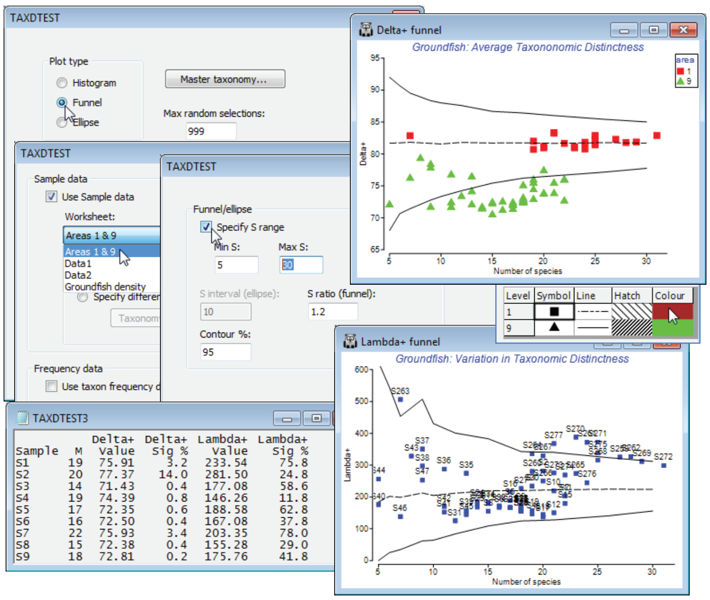
It is impractical to produce detailed histograms, such as those above, for each of the 277 samples, so a preferable option is just to view the 95% lower and upper limits for a range of sample sizes S, using a funnel plot so that a set of samples can be plotted on this. So, first select all sea area 9 (E Central N Sea) and sea area 1 (Bristol Channel) samples from Groundfish density, with Select>Samples>(•Factor levels)>Factor name: area>Levels, leaving only 1 and 9 in the Include box, and Tools>Duplicate this, renaming it Areas 1 & 9 (and remove the selection on the original sheet with Select>All, for later use). Then run Analyse>TAXDTEST again, on Groundfish taxonomy, with (Plot type•Funnel) & (Max. random selections: 999) and Next>(✓Use Sample data>Worksheet: Areas 1 & 9). Now, Next>(Funnel/ellipse✓Specify S range)>(Min S: 5) & (Max S: 30), to span the spread of S values on the display. The (S ratio (funnel): 1.2) option determines how many S values are calculated in the range 5 to 30, the S values stepping up by multiples of 1.2 by default (then rounded), thus S = 5, then 6 (=5$\times$1.2) etc. The final box on this screen gives 95% intervals if the default is taken (2.5% of simulations fall above the upper limit and 2.5% below the lower limit).
The results and funnel plots for $\Delta^{\scriptscriptstyle +}$ and $\Lambda^{\scriptscriptstyle +}$ are shown below and indicate that, whilst area 1 samples are within expected ranges for average taxonomic distinctness, based on the 93 species master list, area 9 samples have reduced diversity (AvTD is the more easily interpretable of the two indices, since it measures the average breadth of the assemblage). Rogers et al 1999 (reference in Section 5) discuss possible reasons for this. Note that these plots have been tidied up, with Graph>Sample Labels & Symbols, by removing the labels and adding symbols for factor area, changing symbol size/colour etc., as for any other plot. The probability limits could be further smoothed by running with (Max random selections: 9999) but will still show kinks for small S, because S is discrete.
Using taxon frequency in simulations
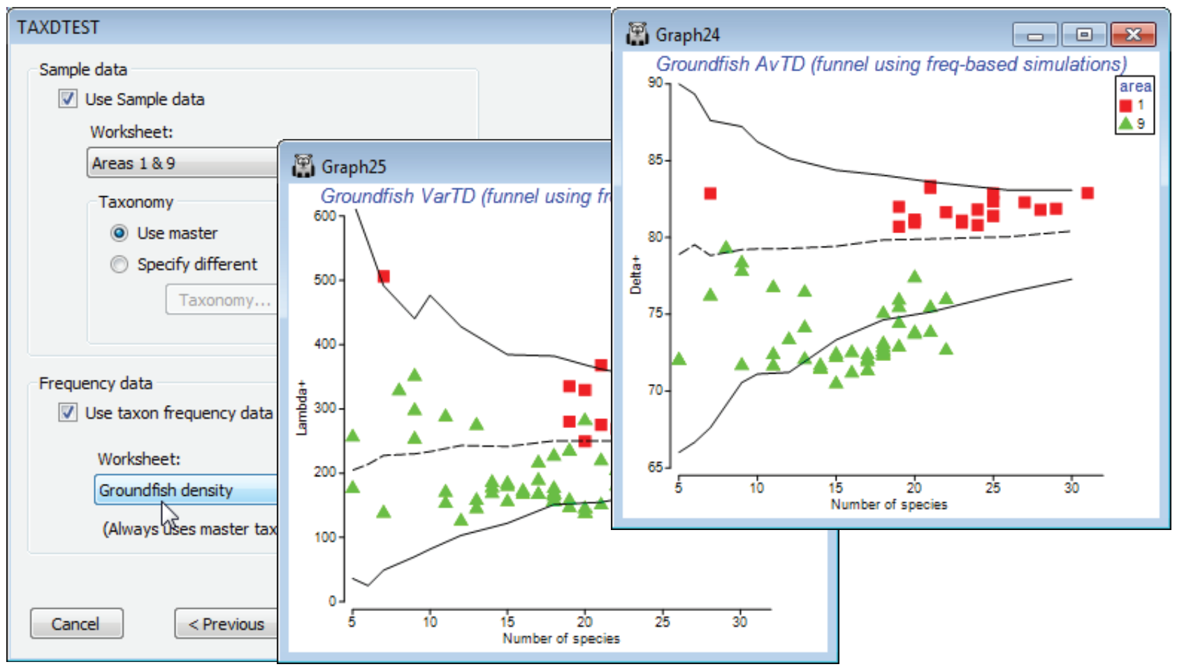
Another option on the TAXDTEST dialogs is that the simulation of random draws from the master list, to generate histograms, funnels etc., can be constrained to match the probabilities of occurrence of each species, as observed in a large set of samples defining those taxon frequencies. Thus certain species are picked more often in the random subsets, because they are observed to be present more often in real samples of this type. The simulated mean and range of (e.g.) AvTD values generated in this way could be argued to give a more realistic yardstick for assessing the observed AvTD. These are produced by checking (✓Use taxon frequency data) and supplying a data matrix (which will be turned into P/A, if it is not already that), with a wide spread of samples of the full set of species in the master taxonomy, which can be used to calculate frequencies of occurrence.
A natural example here would use the full Groundfish density sheet (having removed the earlier selection), with its large number of samples (277) determining probabilities of occurrence of each of the 93 species in any one sample. Now run Analyse>TAXDTEST on Groundfish taxonomy, again with (Plot type•Funnel), the default taxonomy options and (✓Use Sample data)>(Worksheet: Area 1 & 9), as before, but with (✓Use taxon frequency data)>(Worksheet: Groundfish density). Specifying S ranges as previously produces the plot shown below, in which the frequency-based simulated mean is no longer exactly independent of the sub-list size s, though the increase with s is seen to be slight here, on the scale of the probability limits, and the conclusions would be largely the same. Of course, the real $\Delta^{\scriptscriptstyle +}$ values are unchanged – they are not a function of assumptions made about the relevant master list to simulate from, or whether to carry out simple random or frequency-based simulations. And naturally, if your study does not lend itself to testing hypotheses about assembly rules of species drawn from any sort of regional master list, you can simply use the taxonomic indices in the same way as demonstrated earlier for a range of diversity measures, in a purely comparative way across a series of groups, in univariate means plots or ANOVA tests based on the replicate information. (E.g. you can select a single measure, such as $\Delta^{\scriptscriptstyle +}$, and take Euclidean distances on its 277 values across all rectangles here, inputting that resemblance matrix to the PERMANOVA routine in the PERMANOVA+ add-on, to give exactly the ANOVA table for a one-way test of the area factor, with the F value tested by permutation, not F distribution tables).
‘Ellipses’ for joint values of ($\Delta^{\scriptscriptstyle +}$, $\Lambda^{\scriptscriptstyle +}$))
The final option is to consider $\Delta^{\scriptscriptstyle +}$ and $\Lambda^{\scriptscriptstyle +}$ in combination, by plotting 95% probability contours for their joint distribution, under the null hypothesis of simple random (or frequency-based) selection from the master species list. Optionally, pairs ($\Delta^{\scriptscriptstyle +}$, $\Lambda^{\scriptscriptstyle +}$) from a real sample data matrix can be added. There may be some advantage in looking at both measures simultaneously because departures from expectation may reveal themselves as, say, lowish $\Delta^{\scriptscriptstyle +}$ and highish $\Lambda^{\scriptscriptstyle +}$ values, neither of which was significant on its own, but in combination outside the joint ($\Delta^{\scriptscriptstyle +}$, $\Lambda^{\scriptscriptstyle +}$) contours, for which $\Delta^{\scriptscriptstyle +}$ and $\Lambda^{\scriptscriptstyle +}$ might be negatively correlated. (The contours are drawn by approximating the simulations by a bivariate normal distribution in a transformed space, then back-transforming – Chapter 17, CiMC).
Just in order to create an example of how TAXDTEST can be run from a variable similarity matrix (such as might be found in a functional rather than taxonomic description of species relatedness, thus creating an Average Functional Distinctness diversity, AvFD, see Somerfield et al 2008, ICES J Mar Sci 65: 1462-1468), take Analyse>Similarity>(•Taxonomic), which simply returns a matrix of distances through the taxonomic tree. With this (Resem2) as the active window, run Analyse>TAXDTEST with option (Plot type•Ellipse) & (✓Use Sample data>Worksheet: Area 1 & 9) & (✓Specify S range)>(Min S: 10) & (Max S: 30) & (S interval (ellipse): 5), and selecting simple random sampling, i.e. uncheck (✓Use taxon frequency data). With (Contour %: 95), five contours will be produced, within which approximately 95% of the $\Delta^{\scriptscriptstyle +}$, $\Lambda^{\scriptscriptstyle +}$) pairs will lie, for s = 10, 15, 20, 25 and 30 random species draws. These contours must logically be concentric – if they do not look so it is certainly worth specifying more simulations, e.g. by (Max random selections: 9999) on the first TAXDTEST dialog screen. You may need to change the symbol types/colours again to get the first plot below, depending on which part of the Explorer tree you made the change to the Key area previously (if it was in the Area 1 & 9 sheet itself then this will be retained). There will now also be a key which controls the line type and line/shading colour for the 95% contours, and though this can be accessed from the Keys tab on the Graph Options dialog box, if changes are needed it is simplest just to click on the line key in the plot itself, taking you into the colour dialog.
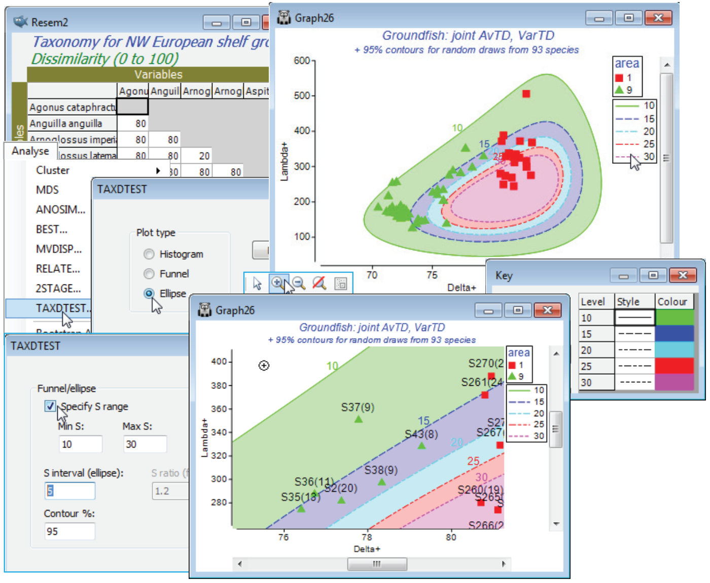
For each sample, the idea is to visually interpolate between the contours for the two s values that straddle its observed number of species S, and determine whether that point is inside or outside its expected 95% contour (a Bonferroni-type correction could be used for the probability limits, or you should just bear in mind in interpreting the plot that 1 in 20 of points will fall outside 95% limits under random draws!). The conclusion here is again of a lower than expected average taxonomic distinctness (but mid-range VarTD) for area 9, and this is discrete from area 1, which has expected mid-range AvTD (and little evidence of VarTD being higher than expected). The interpretation of $\Delta^{\scriptscriptstyle +}$ and $\Lambda^{\scriptscriptstyle +}$ in general is covered in Clarke KR & Warwick RM 2001, Mar Ecol Prog Ser 216: 265-278 and Warwick RM & Clarke KR 2001, Oceanog Mar Biol Ann Rev 39: 207-231, and this study specifically in Rogers et al 1999, J Anim Ecol 68: 769-782 and Chapter 17 of CiMC.