2. Factors (and Indicators), identifying sample (and species) groups
- Active window
- Use of factors
- Creating & filling in factors
- Cut, Copy, Paste, Delete in factors
- Renaming & reordering factors
- Multiple sessions and recent workspaces
- Combining factors (e.g. to average)
- Factor keys
- Importing factors
- Label matching
- Factors in *.xls(x) or *.txt files
- Creating indicators on variables
- Indicators in selection
- Variable information (aggregation files)
Active window
If you have been carrying out the manipulations in Section 1, by now you will have several sheets open in the C:\Examples v7\Tasmania workspace, the worksheet Tasmania nematodes and several identical versions of the copepod assemblages. Unclutter your PRIMER desktop by Window> Close All Windows and then re-display just Tasmania nematodes and Tasmania copepods by clicking on their icons in the Explorer tree. (If the workspace is clear, then File>Open these two *.pri files). It is fundamental to operation of PRIMER that only one window in the workspace is considered active at any one moment, and this will always be displayed on the PRIMER desktop and be identified by the slightly deeper colour title bar and the highlighted entry in the Explorer tree. You can select which one to activate by clicking anywhere on its window or the entry in the tree. Menu selections apply only to the active window, e.g. File> Save As, Edit>Labels, and the Analyse and Tools items (though these may specify one or more secondary sheets needed for a composite analysis). Note also that menus are dynamic, with content that changes with the context. When the active window is a rectangular data sheet, different Analyse options (e.g. Resemblance, DIVERSE, PCA) are available than for a triangular resemblance matrix (e.g. CLUSTER, MDS).
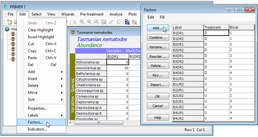
Use of factors
With Tasmania nematodes as the active window, select Edit>Factors from the main menu (or use the shortcut right click when the cursor is over the data matrix to bring up a combination mainly of the Edit and Select menus), and observe that there are already two factors defined. The treatment factor Treatment splits the 16 Tasmanian sandflat samples into two levels, namely whether they are from disturbed (D) or undisturbed (U) areas of sediment. The Block factor divides the samples up in a different way, into four levels, the four separate sampling patches across the sandflat (1 to 4). In statistical terminology, the treatment and block factors are crossed, meaning that there are samples at every combination of levels of the first and second factors. Factors are heavily used throughout PRIMER, in at least two main ways:
a) to define a group structure for multivariate hypothesis testing (e.g. ANOSIM, see Chapter 6 of the CiMC manual). Such a priori structuring of the samples (i.e. prior to seeing the data) plays an important role in formal inference about sample patterns, and also the interpretation of which variables (e.g. species) are primarily responsible for distinguishing specific groups (Chapter 7);
b) purely as a means of labelling points on plots, in dendrograms etc., in which case there might be a different ‘level’ for every sample, e.g. a fuller or more abbreviated site name than is held in the sample label. There is no limit on the length or alphanumeric content of a factor level.
Factors are carried around and saved as part of the data sheet they are linked to, and not saved as separately named data sheets. This is in contrast to (numeric) environmental variables associated with each biological sample, which are held in a separate sheet – preferably with the same sample labels as the biota, and which could have some or all of the same (categorical) factors defined. To emphasise that block designation is purely a category here, not a numeric sequence, a new factor Blk will be added here, with levels B1, B2, .. not 1, 2, … (as seen in the previous text file versions).
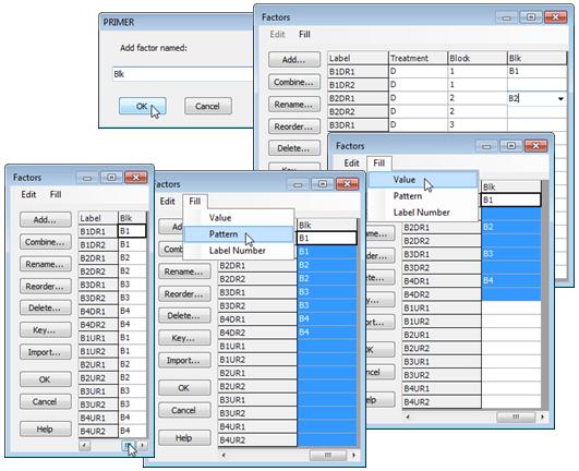
Creating & filling in factors
In the Factors dialog box (obtained from Edit>Factors on Tasmania nematodes) take Add>(Add factor named: Blk). The cursor is then at the top of the new (blank) label column, ready to start typing. You need only put in the first entry for each new level (B1, B2, ..) if they are in groups of identical values. (There are only two replicates per cell here so only pairs of identical values, and it is just as quick to type them all, but this new feature in PRIMER 7 will typically save much typing of identical strings, so is demonstrated below). Having entered B1, B2, B3, B4 in the relevant rows (1, 3, 5, 7), highlight the first 8 entries and take Fill>Value, which fills in the blanks in the top half. (For any run of blank entries in the highlighted area, Fill>Value will simply repeat the last filled entry immediately above them). The same sequence then needs to be generated for the second set of 8 entries and this is quickly achieved by highlighting the whole column, clicking on its label (Blk), then taking Fill>Pattern. (This copies any run of fully filled entries into any blank entries starting immediately below them, stopping part way through if necessary, if it gets to another filled entry – filled entries are never overwritten – and then repeating this through the highlighted area).
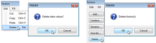
Cut, Copy, Paste, Delete in factors
An alternative (and clumsier!) way of creating this factor would be type in the top half, then highlight and Edit>Copy these 8 entries and Edit>Paste them when the cursor is at the start of the lower set. (Pasting does, of course, overwrite existing entries, as in normal Windows practice). The usual Cut, Copy, Paste and Delete operations can be performed with key strokes (Ctrl-X, Ctrl-C, Ctrl-V and Del key), rather than from the Edit menu, in a fully standard way throughout PRIMER. Deletes will trigger a query of ‘Delete data values?’ because there is no Undo option on the Factors dialog. If a significant deletion takes place accidentally, the best strategy is to abort any changes made to the factors sheet since it was entered on this occasion, by the Cancel button (which again throws a query box of ‘Cancel all changes?’), and you can reopen the factors sheet and try again.
Do not confuse deleting factor entries with removing the whole factor (or several factors) from the factor sheet. The latter can be achieved by highlighting the factor – clicking on its label at the top of the column (or clicking and dragging to capture several consecutive factors) – and taking the Delete button on the left of the dialog box. Try this out by deleting the (now redundant) Block factor. This also generates a query box, this time of ‘Delete factors?’ not ‘Delete data values?’.
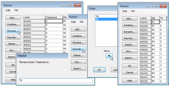
Renaming & reordering factors
Finally, to make factors in the Tasmania nematodes sheet consistent with the text format copepod files of Section 1, rename the Treatment factor as Trt using Rename>(Rename factor Treatment to: Trt), and rearrange the order of factors to put Blk first, with Reorder clicking on Blk and Move$\uparrow$.
Multiple sessions and recent workspaces
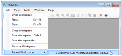
As a further example of Fill>Value to quickly set up a factor of group levels you might like to re-open the saved workspace from the oil-field study of Section 1, Ekofisk ws.pwk. Taking File>Open and supplying the workspace name from the directory C:\Examples v7\Ekofisk macrofauna would lead to a prompt to save the currently active Tasmania workspace prior to shutting it down, in order to open the Ekofisk workspace. If it is useful to have both sets of data being open and worked on at the same time (though independently), a different solution is needed. This is generally not to open Ekofisk data files into the Tasmania workspace – data sets that will never interact in a common analysis are best kept in separate workspaces – but to launch multiple runs of PRIMER. These will not interfere with each other: a copy is taken of the current version of each file at the time it is loaded into the workspace, so the original file is never then modified by internal workspace actions or saving the workspace (only explicitly taking Save Data As and providing the same file name can alter the original file’s contents, and even this requires a confirmation stage before it is over-written). In this second PRIMER desktop therefore, re-open the Ekofisk workspace with File> Recent Workspaces>C:\Examples v7\Ekofisk macrofauna>Ekofisk ws.pwk.
Now take Edit>Factors>Add>(Add factor named: Dist#) in order to match the alphabetic codes for the different distance groups of sites from the oil-field centre: D, B, C, A with numeric ones: 1, 2, 3, 4 respectively. (This will be needed for a later example when it is useful to treat this factor as ordered categorical – PRIMER does not treat alphabetic levels in factors as providing an ordering). As previously, only a 1 in the first row (site S30), a 2 in the S27 row, a 3 opposite S4 and a 4 at S18 need to be typed in, then highlight the column and Fill>Value. Another simple example of the use of Fill would be to produce a continuous ordering of distances from the oil-field centre, by adding a new blank factor Dist order, then highlighting and filling it with Fill>Value>Label Number, since here the sample rows in the file have already been ordered by increasing distance from the field.
Resave the workspace by File>Save Workspace – there is no prompt for a workspace name this time since it has already been saved as Ekofisk ws (as can be seen from the top line of the Explorer tree). Saving to a different workspace name requires File>Save Workspace As. You can now exit this PRIMER session with File>Exit but note that the previous PRIMER session on the Tasmania meiofauna data remains open, and we will use this to look at the remaining Factor dialog options.
Combining factors (e.g. to average)
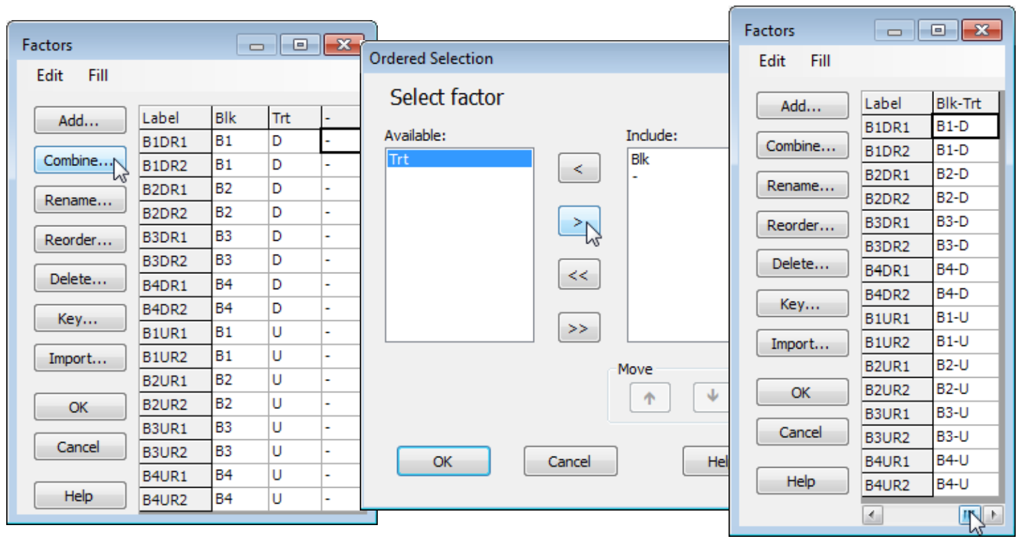
With the Tasmania nematodes sheet active, open the Factors dialog with Edit>Factors. Combining factors (Combine) can be a quick and effective way of creating new factors or composite sample names in nested or crossed layouts. Firstly, though, it is usually useful to create a separator ‘factor’ (or perhaps more than one), by Add>(Add factor named: -), filling the column with dash symbols, by entering a dash in the first row, highlighting the factor and using Fill>Value again. Combine now displays a typical selection box (PRIMER uses a similar dialog for many other analyses, e.g. selecting a subset of the data by levels of a factor). Click on Blk and ![]() , then -
, then - ![]() and Trt
and Trt ![]() , to set up which factors are to be combined and in what order. (Note that the double arrows
, to set up which factors are to be combined and in what order. (Note that the double arrows
![]() move all items from the (Available) list to the (Include) list, or back, and a selection of entries can be moved in one operation by holding the Ctrl key down as the items are clicked – or the Shift key to obtain a range of items – as in usual Windows practice). Pressing OK then gives a composite factor with name Blk-Trt and the 8 levels: B1-D, B2-D, …, B4-D, B1-U, …, B4-U, which are the 8 cells of the two factor crossed design, with two replicates at each level.
move all items from the (Available) list to the (Include) list, or back, and a selection of entries can be moved in one operation by holding the Ctrl key down as the items are clicked – or the Shift key to obtain a range of items – as in usual Windows practice). Pressing OK then gives a composite factor with name Blk-Trt and the 8 levels: B1-D, B2-D, …, B4-D, B1-U, …, B4-U, which are the 8 cells of the two factor crossed design, with two replicates at each level.
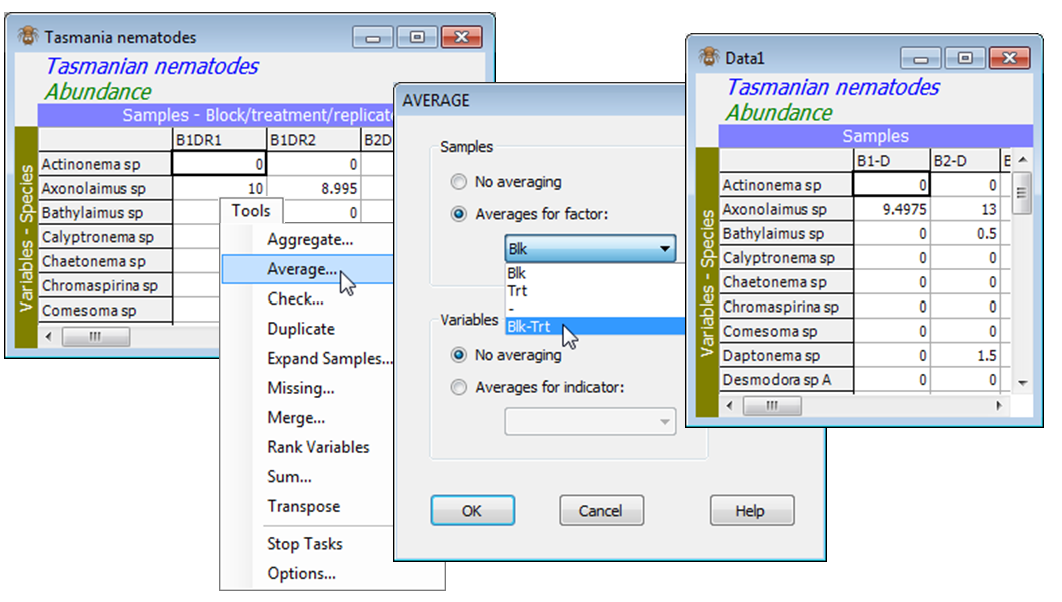
Such a combined factor has several uses, e.g. it can be a composite label on an ordination plot, and it is essential for averaging over the replicates in the data, to obtain a matrix of mean values, for each of the 8 block $\times$ treatment combinations here. This is simply achieved with an OK for all the changes you have made to the Factor information, and then Tools>Average>(Samples•Averages for factor: Blk-Trt) & (Variables•No averaging). This creates a new data sheet, Data1, in which the sample labels are the levels of the combined Blk-Trt factor, as seen above (B1-D, B2-D, etc). It also carries across what factor information it can from the original sheet (take Edit>Factors on Data1), though a factor for which different levels have been averaged over will have ‘Undefined!’ entries (e.g. produce averages for factor Trt, and the Blk factor entries would all be undefined, naturally).
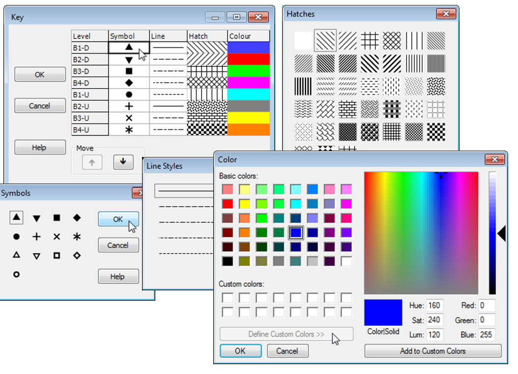
Factor keys
Importing factors
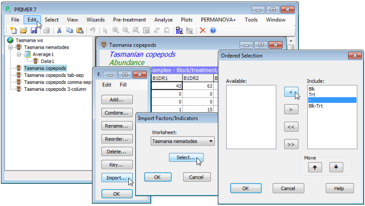
New factors can be created at several stages during an analysis, not just when the active window is a data sheet (e.g. from a resemblance matrix or even a plot) and the new information is propagated both forwards and backwards through the same branch on the Explorer tree. (There are exceptions to backward propagation, in cases where an action, such as Tools>Average or Sum, fundamentally restructures the samples – existing factors are propagated forward through these steps but not back, understandably). However, when two sheets are in the same workspace but otherwise unconnected (e.g. they are on branches from different initial data sheets), factor information which applies to the sample label names which they share can be transferred between them using the Import button on the Factors dialog. An example is the Tasmania copepods(.pri) sheet, which should already be open in the Tasmania workspace. Edit>Factors shows that it currently has no factors defined, but its samples (and, importantly, their labels) are identical to those for the nematode data sheet. Taking Import>(Worksheet: Tasmania nematode) & (Select) gives a selection box, which should list the three factors that were created for the nematode data: Blk, Trt and Blk-Trt. Any factors that are not needing transfer are excluded just by moving them, with ![]() , from the Include: to the Available: box (you might like to do this with the separator column ‘-‘). Then take OK on this and the next two boxes, and the desired transfer of three factors to the Tasmania copepod data sheet will occur.
, from the Include: to the Available: box (you might like to do this with the separator column ‘-‘). Then take OK on this and the next two boxes, and the desired transfer of three factors to the Tasmania copepod data sheet will occur.
Label matching
Alternatively, the same endpoint could have been achieved by Adding three new blank factors to the copepod sheet and copying and pasting the contents of the Blk, Trt and Blk-Trt columns from the nematode factor sheet. If importing entries from an external source, such as an Excel column, this approach may sometimes be necessary but it is only appropriate when the samples are in the same order in the two data sets (as they are here). In contrast, Import operates by matching up the sample labels in the two files and can therefore re-order the factor levels appropriately when the samples are in a different order. This is a general feature of PRIMER 7 – a lot of use is made of label matching across data sets in this way, which is why it is vital that labels are defined uniquely within a set and carefully checked for consistency of spelling across sets. Of course, if the two sets of sample labels are not identically defined, but do refer to the same set of samples, in the same order, then a copy and paste of the factor content is the only way of transferring the factors.
Factors in *.xls(x) or *.txt files
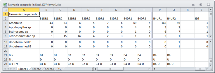
As noted in Section 1, factors can be created as part of the Excel or text files which are the usual means of inputting data to PRIMER 7. Similarly, data sheets that are saved from PRIMER to Excel (*.xls or *.xlsx) or text (*.txt) formats will automatically export the factors also. The principle is that, when the data has samples as columns, any factors are placed in the input or output sheet as additional rows at the bottom of the array, separated from the data by a blank row. If samples are rows, factors are held as columns to the right of the array, again after a blank column. The ‘record’ text format differs slightly: after the 3-columns (sample label, variable label, data value) comes a blank column and factor levels (then possibly a blank column and indicator levels – see below).
Take File>Save Data As>(Save as type: Excel 2007 Files (*.xlsx)) to output Tasmania copepods in Excel format, and open Excel to examine the form in which factors are output (and input). Text format versions of the same data (with Blk and Trt factors only) are shown in Section 1.
Creating indicators on variables
Indicator is the term PRIMER uses for a factor defined on the variables not on the samples. It is convenient to use a separate term because ‘factor’ has a well-established statistical meaning (e.g. in ANOVA-type layouts), and refers to structures defined on samples, not on variables. Indicators are less used than factors in practice, though they have a useful role in selecting or removing subsets of variables for the analysis of samples (e.g. only analyse the metals data rather than all environmental variables; only analyse zooplankton, omitting phytoplankton species etc.). Adding and manipulating indicators, however, proceeds exactly as for factors, with parallel choices of Add, Combine, Rename, Reorder, Delete, Key and Import from the Indicators sheet produced by Edit>Indicators.
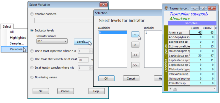
A simple example is seen in the Tasmania copepods(.pri) data sheet. Edit>Indicators (also on the right click menu when the cursor is over the data sheet) shows the indicator ID?, which records whether each taxon has been identified (1) or is an undetermined specimen (0). The ID? indicator is also shown above (far right) in the Excel format of this file.
Indicators in selection
Selection by indicator levels is demonstrated by Select>Variables>(•Indicator levels)>(Indicator name: ID?)>Levels>(Include: 1) & (Available: 0), giving a subset of the Tasmania copepods data sheet which drops the undetermined species. Of course, for such a small data set there are simpler ways of dropping these last five species – see the range of selection options in Section 3.
Now reverse the selection by Select>All (and Edit>Clear Highlight if you wish), and resave the Tasmania ws.pwk workspace, using File>Save Workspace, for use in later sections.
One apparently obvious application for indicators is to specify which species belong to which higher-order taxonomic groups. If separate multivariate analyses are required by major phyletic group, for example, then the different phyla should be set up as an indicator on the species, since this will allow easy selection of the species in a single phylum from the samples $\times$ species sheet.
Variable information (aggregation files)
However, the full range of hierarchical indicators represented by a Linnaean classification (which species belong to which genera, which genera to families, families to orders, etc.) are usually also best held separately, as a different type of array – that of variable information. Mainly for historical reasons these are termed ‘aggregation files’ in PRIMER, since their initial use was for aggregating species abundances up to genus, family, order, … level information, to judge the extent of change to the interpretation of analyses under coarser identification of taxa (see Chapter 10 of the CiMC manual), and this binary file format is therefore denoted by *.agg. However, in PRIMER 7, arrays of variable information can be more general (and have other Type definitions than Taxa). Former aggregation file formats can be opened and PRIMER 7 outputs the full range of previous types, e.g. Save as type: PRIMER Var Info Files (*.agg) for PRIMER 7 (binary); PRIMER 6 or 5 aggregation files.agg (also binary); and simple Text (*.txt) or Excel (*.xls) (or *.xlsx) sheets. Examples using aggregation files will be seen later (Sections 5, 11, 15) though the simple rectangular format is seen here by opening Groundfish taxonomy.agg from the C:\Examples v7\Europe groundfish directory. Three ways in which it might be used are to: a) aggregate abundance to higher taxa with Tools> Aggregate (Section 11, and Chapter 10 of CiMC); b) compute biodiversity indices based on the relatedness of species in a single sample, e.g. with Analyse>DIVERSE (Section 15, Chapter 17); c) compute resemblance measures between two samples reflecting (higher) taxonomic relatedness of the species found there (Section 5, Chapter 17).
This new variable information sheet (below) permits the non-numeric entries which are essential for a variables $\times$ taxa ‘look-up’ table but also, and newly in PRIMER 7, will carry over several of the general features of sample $\times$ variables arrays, in that indicators defined on the variables can now be carried around with this array. This might permit the aggregation file to hold alternative names for single species, for example, with an indicator that can be used to select only the taxonomic revision relevant to the historic date of collection/identification of the species count matrix. Importantly, it also allows easy selection of aggregation file subsets, e.g. for testing taxonomic distinctness indices against differing ‘master lists’ by region, habitat or faunal group (Chapter 17 of CiMC). The simple indicator in the example below could be used to select only the Osteichthyes (Class# = 2) from the Variable information: Groundfish taxonomy, as well as from the data: Groundfish density(.pri).
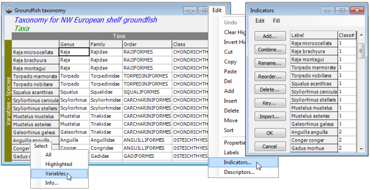
Note the final entry on the Edit menu here. The concept of Descriptors is not particularly relevant to Variable information of type Taxa (they are potentially more relevant to other types of Variable information) but they are the third construction logically needed. Categories (or alternative labels) applied to Samples are termed Factors, when applied to Variables they are called Indicators and when applied to Variable information they are Descriptors.