# 3. Highlighting and selection (Select)
# Highlight and select
There are many cases in which analyses of different subsets of the samples or species are required. This can be easily achieved, without the need to create large numbers of separate datasheets, by temporarily selecting subsets from a single sheet, analysing them (and thus creating new branches on the Explorer tree, with the results windows listing the selection used for any particular branch), and then restoring the full data set. There are several different ways to select subsets, described below, but it is important to keep in mind the distinction between highlighting and selection. The act of clicking on a row and/or column header *highlights* that row and/or column; it does not *select* it. Once you are happy that you have highlighted the correct set of samples (and/or variables) you can select them using the **Select>Highlighted** menu. Highlighting is just an intermediate stage, and has functions other than selection (e.g. to identify samples that need individual transformation, whilst the rest of the matrix remains unchanged - see next section). Alternatively, highlighting can be bypassed altogether and selection made by other direct choices from the **Select** menu.
# (W Australia fish diets)
Dietary data on the gut contents of 7 marine fish species found in nearshore waters of the lower west coast of Western Australia are reported by Hourston M, Platell ME, Valesini FJ, Potter IC 2004, *J Mar Biol Assoc UK* 84: 805-817 and Schafer LN, Platell ME, Valesini FJ, Potter IC 2002, *J Exp Mar Biol Ecol* 278: 67-92. Data is %volumetric gut contribution (reflecting both composition and gut fullness) of each of 39 ‘dietary categories’ (broadly classified taxa), in a total of 68 samples across the 7 fish species (unbalanced replication), each sample being from a pool of 5 fish guts. The data matrix in PRIMER 7 format can be found in C:\Examples v7\WA fish diets\WA fish diets %vol.pri. Since species are involved in the definition of both samples and variables it is important to keep a clear head as to which are which! Here the fish predator species are the sampling device, so different individual fish guts (in pools of 5) constitute the samples. The assemblage studied is the set of prey species (higher taxa) making up the dietary categories; they are the variables.
# Summary Statistics
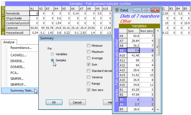
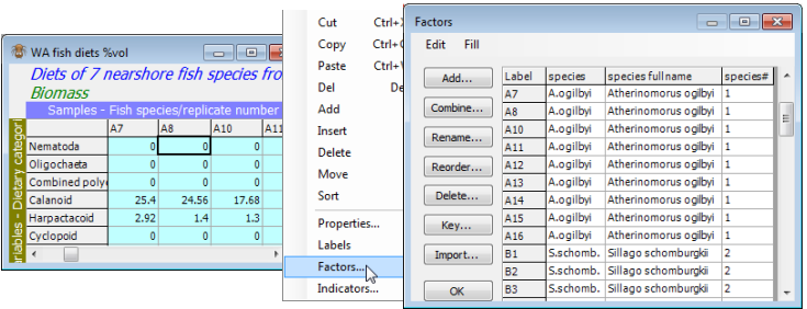
**File>Open**>Filename: WA fish diets %vol, and examine the factors sheet with **Edit>Factors**. The samples form 7 groups (identified in the labels by A to G) which are the different predator species, three of which, B: *Sillago schomburgkii* (*n* = 10), E: *Sillago bassensis* (*n* = 14), G: *Sillago vittata* (*n* = 16), are from the same genus (congeneric) and thus of particular interest in terms of whether their diets are distinguishable (they occupy different niches in the ‘dietary space’). First, calculate simple summary statistics for each sample with **Analyse>Summary Stats**>For•Samples. Not all summary options (Min, Max, Average, Sum, Standard deviation, Variance, Range, Non zero) may be meaningful in particular contexts: one that is informative here is ✓Sum. This shows that three samples (A9, B3 and B4) have low total gut fullness (<<10%), even though from a pool of 5 guts, and it is justifiable to look at the effect of (temporarily) dropping these samples from the analysis on the grounds that they contain little information on dietary composition (and could thus have large variability in similarity with other samples, see Section [5](https://learninghub.primer-e.com/books/primer-v7-user-manual-tutorial/chapter/5-resemblance-similarities-dissimilarities-and-distances) on zero-adjusted Bray-Curtis).
[](https://learninghub.primer-e.com/uploads/images/gallery/2024-05/screenshotpage45a.png)
# Control of highlighting
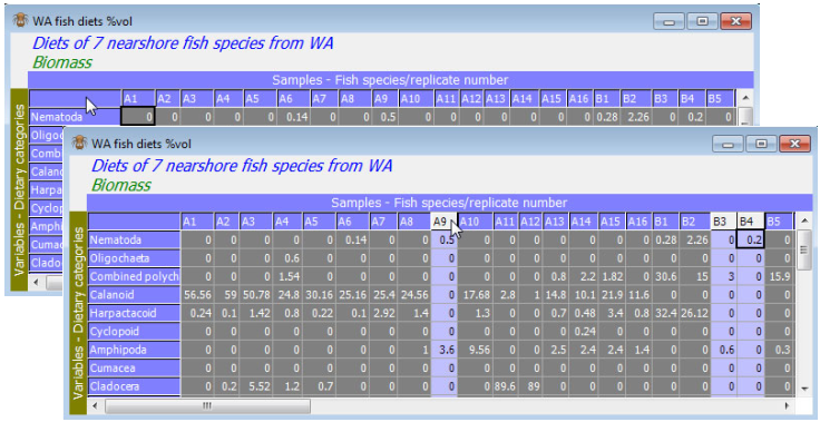
Thus, with the WA fish diets %vol datasheet as the active window, highlight all columns *except* the three samples A9, B3 and B4. There are various ways of doing this. Clicking on a column label highlights that column (in light blue shading if the default Windows colours are used) and is a toggle action (a second click turns off the highlighting). Clicking, holding and dragging the cursor across column headers will highlight a sequence of samples, as will the usual Windows action of clicking on the first, then holding down the Shift key when clicking on the last. (The Ctrl key has no effect; also the toggling action is set so that intermediate columns which are already highlighted will not be turned off if a wider range of columns, including them, are highlighted in these ways). However, the easiest way of highlighting all except a few columns is to highlight all the data, by clicking in the blank cell at the top left of the sheet, then click on the A9, B3 and B4 labels to de-highlight just those. (The top left cell is also a toggle note, so a second click is a convenient way of clearing all highlights, though this can also be done by **Edit>Clear Highlight**).
[](https://learninghub.primer-e.com/uploads/images/gallery/2024-05/screenshotpage46a.png)
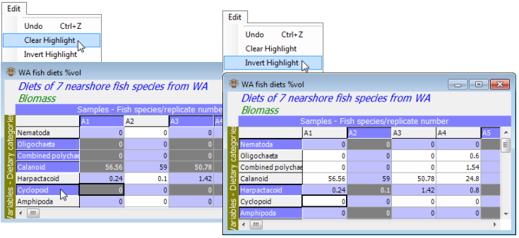
In the default Windows colours, cells in the table have one of three backgrounds: very light grey, light blue or dark grey. Three colours are necessary because highlighting can also be by rows, or rows *and* columns simultaneously. The rule is that the cells with the darkest background are those that are highlighted. You will see this best by turning off all highlights then clicking on a random set of row and column labels: the intersections are considered the highlighted part of the matrix. (Individual cells in the table cannot be highlighted by clicking on them; it is not meaningful to be able to select, say, only A1 Calanoids and B5 Amphipods. It is best not to think of the data as a conventional spreadsheet: only a limited set of operations make sense for sample $\times$ variable arrays). Note that highlights can also be inverted by **Edit>Invert Highlight**.
[](https://learninghub.primer-e.com/uploads/images/gallery/2024-05/screenshotpage46b.png)
# Selecting & deselecting highlights
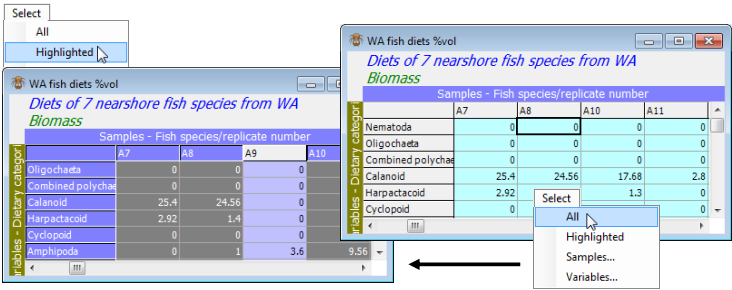
When all except columns A9, B3 and B4 are highlighted, take **Select>Highlighted**. Alternatively, right click when over the data and a drop-down menu will appear, of operations from the **Edit** and **Select** menus, including **Select highlighted**. The matrix entries now have a different (turquoise) background indicating that you are operating with a selection – a new datasheet window is not created and the non-selected data is not lost. The operation can be simply reversed by deselecting the highlight with **Select>All** – the highlights are retained so it is easy to change some of them (or reverse them with **Edit>Invert Highlight**, see example above) and reselect.
[](https://learninghub.primer-e.com/uploads/images/gallery/2024-05/screenshotpage47a.png)
# Duplicating a selected worksheet
Though most Save operations are on whole workspaces, occasionally a data matrix needs to be saved externally, perhaps because it is needed in a different workspace or with other software. In order to protect against overwriting an original, external, data file with a version which is under a (possibly temporary) selection, **File>Save Data As** will ignore selections and save the whole data. To force a save of only the selection, you must first duplicate the selected sheet, with **Tools> Duplicate**. Do this on the selected form of the WA fish diets %vol data – which has excluded A9, B3, B4 – to create a new datasheet, Data2, which will now not contain these samples when saved.
# Selecting by factor levels
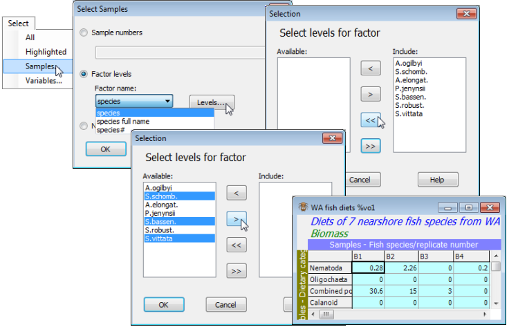
The highlighting route to selection can be bypassed altogether using the other options on the **Select** main menu, **Select>Samples** and **Select>Variables** (and an example of the latter was seen in the previous section). Here, to select only those samples from the three congeneric *Sillago* predator fish species (labels starting B, E or G), it would be neater to use the factors that have already been set up to identify these different levels: S.schomb., S.bassen., S.vittata from the factor species, or the non-abbreviated species full name factor, or equally, 2, 5 and 7 from the numeric factor species#.
[](https://learninghub.primer-e.com/uploads/images/gallery/2024-05/screenshotpage47b.png)
From the WA fish diets %vol datasheet, take **Select>Samples**>•Factor levels>(Factor name: species)>**Levels**, giving a standard Selection window, with boxes listing levels to Include, and those Available but not included. Move back all items to the Available list with  , then using the
  button move back the desired levels: S.schomb., S.bassen., S.vittata to the Include list. This can be either singly, or all of them can be highlighted with Ctrl clicks (a range would use Shift click), in the usual Windows manner, and then all taken across to the Include box with .
[](https://learninghub.primer-e.com/uploads/images/gallery/2024-05/screenshotpage48a.png)
# Multiple selections
It is important to note the effect of this second selection on WA fish diets %vol; it produces a sheet of all samples from these three *Sillago* species. The prior exclusion of samples A9, B3 and B4 has been ignored – each new selection is a fresh operation on the full data array that is held in that worksheet. If, as seems likely, a compounding of the two selections was required, then that is easily achieved, in at least two ways. One would be to take the current selection (all B, E and G samples), highlight everything displayed (e.g. by clicking in the blank, left corner box), dehighlight B3 and B4, by clicking on their column labels, then **Select>Highlighted**. (This is logically sound because all the omitted A, C, D, F samples from the first selection are not highlighted at that point.) This would retain the single copy of WA fish diets %vol in the Explorer tree. A more general option though, which would be more relevant to a complex multiple sequence of selections, is simply to **Tools>Duplicate** the sheet after every selection, then do the next selection on the new sheet. So, if the above selection of the *Sillago* samples had taken place on Data2, samples B3 and B4 would automatically have been excluded. Note, however, that if the two selections are on different axes (selecting a subset of both samples and variables) then they will not interfere with each other, i.e. when sequentially taking **Select>Samples**>•Factor levels and **Select>Variables**>•Indicator levels.
A third option for repeated selection of samples, with the outcome of multiple selection being a single worksheet (rather than a series of copies), is to create a compound factor (with **Factors> Combine**), which will allow simple selection of one (or more) of its levels.
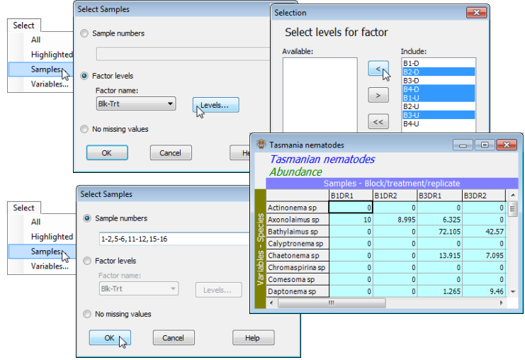
To illustrate this, save and close down the above workspace, as WA fish ws(.pwk), and re-open the previous workspace, C:\Examples v7\Tasmania meiofauna\ Tasmania ws. Here there are only 16 samples, which helps for illustrative purposes (though in the real context would make selections quickest by simple highlighting). The study design has two crossed factors: *Trt* (disturbed, D, and undisturbed, U, sediment patches), and *Blk* (4 areas of sand-flat, B1 to B4), with 2 replicates in each combination. An example of 2-factor selection for the Tasmania nematodes sheet would be to select distinct sand patches within each treatment, say blocks 1 and 3 for D, and blocks 2 and 4 for U (which would make the data sheet 2-factor nested rather than crossed). Use the *Blk-Trt* combined factor created in the previous section to **Select>Samples**>•Factor levels>(Factor name: Blk-Trt)> **Levels**, leaving B1-D, B3-D, B2-U, B4-U in Include and moving the others back to Available.
# Selecting by number and non-missing
It may sometimes be easier to use the sample numbers, here **Select>Samples**>•Sample numbers> 1,2,5,6,11,12,15,16, though this is more likely to be useful where such numerical lists are output in results (e.g. by the BEST routine, Section [13](https://learninghub.primer-e.com/books/primer-v7-user-manual-tutorial/chapter/13-linking-assemblage-to-environment-best-bio-env-linktree)), and can be copied and pasted into this dialog box.
[](https://learninghub.primer-e.com/uploads/images/gallery/2024-05/screenshotpage49a.png)
The final possibility is **Select>Samples**>(•No missing values) in which only those samples which have no entries of
button move back the desired levels: S.schomb., S.bassen., S.vittata to the Include list. This can be either singly, or all of them can be highlighted with Ctrl clicks (a range would use Shift click), in the usual Windows manner, and then all taken across to the Include box with .
[](https://learninghub.primer-e.com/uploads/images/gallery/2024-05/screenshotpage48a.png)
# Multiple selections
It is important to note the effect of this second selection on WA fish diets %vol; it produces a sheet of all samples from these three *Sillago* species. The prior exclusion of samples A9, B3 and B4 has been ignored – each new selection is a fresh operation on the full data array that is held in that worksheet. If, as seems likely, a compounding of the two selections was required, then that is easily achieved, in at least two ways. One would be to take the current selection (all B, E and G samples), highlight everything displayed (e.g. by clicking in the blank, left corner box), dehighlight B3 and B4, by clicking on their column labels, then **Select>Highlighted**. (This is logically sound because all the omitted A, C, D, F samples from the first selection are not highlighted at that point.) This would retain the single copy of WA fish diets %vol in the Explorer tree. A more general option though, which would be more relevant to a complex multiple sequence of selections, is simply to **Tools>Duplicate** the sheet after every selection, then do the next selection on the new sheet. So, if the above selection of the *Sillago* samples had taken place on Data2, samples B3 and B4 would automatically have been excluded. Note, however, that if the two selections are on different axes (selecting a subset of both samples and variables) then they will not interfere with each other, i.e. when sequentially taking **Select>Samples**>•Factor levels and **Select>Variables**>•Indicator levels.
A third option for repeated selection of samples, with the outcome of multiple selection being a single worksheet (rather than a series of copies), is to create a compound factor (with **Factors> Combine**), which will allow simple selection of one (or more) of its levels.
To illustrate this, save and close down the above workspace, as WA fish ws(.pwk), and re-open the previous workspace, C:\Examples v7\Tasmania meiofauna\ Tasmania ws. Here there are only 16 samples, which helps for illustrative purposes (though in the real context would make selections quickest by simple highlighting). The study design has two crossed factors: *Trt* (disturbed, D, and undisturbed, U, sediment patches), and *Blk* (4 areas of sand-flat, B1 to B4), with 2 replicates in each combination. An example of 2-factor selection for the Tasmania nematodes sheet would be to select distinct sand patches within each treatment, say blocks 1 and 3 for D, and blocks 2 and 4 for U (which would make the data sheet 2-factor nested rather than crossed). Use the *Blk-Trt* combined factor created in the previous section to **Select>Samples**>•Factor levels>(Factor name: Blk-Trt)> **Levels**, leaving B1-D, B3-D, B2-U, B4-U in Include and moving the others back to Available.
# Selecting by number and non-missing
It may sometimes be easier to use the sample numbers, here **Select>Samples**>•Sample numbers> 1,2,5,6,11,12,15,16, though this is more likely to be useful where such numerical lists are output in results (e.g. by the BEST routine, Section [13](https://learninghub.primer-e.com/books/primer-v7-user-manual-tutorial/chapter/13-linking-assemblage-to-environment-best-bio-env-linktree)), and can be copied and pasted into this dialog box.
[](https://learninghub.primer-e.com/uploads/images/gallery/2024-05/screenshotpage49a.png)
The final possibility is **Select>Samples**>(•No missing values) in which only those samples which have no entries of Missing! for any of their variables will be selected. Missing! entries are unlikely for species matrices (as here) but this facility might be useful sometimes for environmental arrays, to find samples which have a complete set of variables.
# Selecting variables
Any of the options for selecting samples are also available for selecting variables, e.g. selecting by variable numbers or by levels of an indicator, the latter as seen in the example of the previous section, in which the Tasmanian copepods of ‘Undetermined taxa’ were excluded. There is a similar construction of selecting variables with no Missing! entries across the full set of samples. Note that if the selection option of (•No missing values) is chosen for both samples and variables, the order in which these are taken will affect the outcome. In practice, if it is required to form a complete matrix (and this is now less essential than in previous versions of PRIMER since all resemblance measures are now defined under pairwise-elimination of missing values, Section [5](https://learninghub.primer-e.com/books/primer-v7-user-manual-tutorial/chapter/5-resemblance-similarities-dissimilarities-and-distances)), a more careful manual deselection of the array rows and columns is likely to be preferable, utilising knowledge of which are the most important samples or variables to attempt to retain. Alternatively, where the data can be approximated by multivariate normality, missing entries can sometimes be successfully estimated by the EM algorithm – see the **Tools>Missing** menu, in Section [12](https://learninghub.primer-e.com/books/primer-v7-user-manual-tutorial/chapter/12-analysing-environmental-variables-draftsman-plot-pca).
# Selecting by ‘most important’
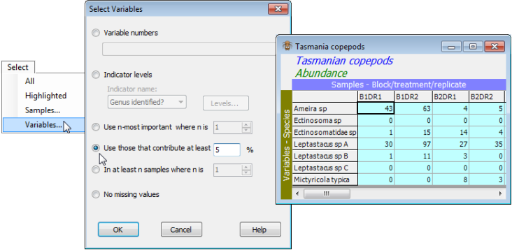
There are, however, three other selection methods under **Select>Variables** that are specific to selecting species (or other taxon-type) variables, in which matrix entries are positive ‘amounts’ of that species (counts, biomass, area cover etc.). The idea of the first two options is to be able to drop species which are not a substantial component of the overall counts (or biomass, area cover etc.) in any sample. The third option, an addition to PRIMER 7, is to drop species which occur in fewer than a specified number of samples, e.g. **Select>Variables>**(•In at least *n* samples where *n* is 2) would drop species which were only seen on one occasion. (It is important to note, however, that removing low abundance or rare species in this way is not required for most of the methods in PRIMER, based on Bray-Curtis similarities for example, and should be done only where there is good reason, e.g. when using a resemblance coefficient which is sensitive to rare species – such as chi-squared distance or Gower, Section [5](https://learninghub.primer-e.com/books/primer-v7-user-manual-tutorial/chapter/5-resemblance-similarities-dissimilarities-and-distances)). The option to **Select>Variables>**(•Use those that contribute at least 5 %) applied to the copepod counts in Tasmania copepods would drop species which, for every sample, account for <5% of its total abundance, leaving only 7 of the original 17 species in the selected sheet. Alternatively, the number of species to retain can be specified, rather than the %, but the principle is the same. Taking **Select>Variables>**(•Use *n*-most important where *n* is 7) generates the same set of species, naturally. If *n* is larger, say 10, then to be retained, the threshold percentage that a species must contribute somewhere will drop – in fact a threshold of around 3% will leave 10 species. If *n* is smaller, say 5, then a higher percentage cut-off is needed (10% in fact). The algorithm simply varies the cut-off percentage until the matrix retains only the exact number of species *n* requested. This means of selecting ‘important’ species (rather than by taking their total abundance across all samples and selecting the top *n*-ranked of those) is preferable because it retains species which are important in impoverished sites, with low total abundance.
[](https://learninghub.primer-e.com/uploads/images/gallery/2024-05/screenshotpage50a.png)
The point is re-iterated that **Select>Variables** will operate in combination with **Select>Samples** (unlike repeated **Select>Samples** or **Select>Variables** operations on their own), to ensure the behaviour that would be expected. That is, if a sample selection is in operation then the ‘most important’ 10 species – or the species which occur in at least 2 samples – are determined only with regard to that selection, not using all the samples.
Close the Tasmania ws – there is no need to resave it, since when met in a later section it will not be for a subset of either the samples or species.
# Selection in resemblance matrices
Looking ahead to Section [5](https://learninghub.primer-e.com/books/primer-v7-user-manual-tutorial/chapter/5-resemblance-similarities-dissimilarities-and-distances), when the active window is a (triangular) resemblance matrix, selection can take place just as for a (rectangular) datasheet, by **Select>Highlighted** or **Select>Samples>**(•Sample numbers) or (•Factor levels). Another option is provided in that case: selection of only the rows and columns containing at least one value above or below a specified threshold by, for example, **Select>Samples>**(•Values>0.95), or selecting only rows and columns containing at least one Undefined! resemblance entry, by **Select>Samples>**(•Undefined values). These are mainly used for picking out, in the first case, collinear environmental variables from a large correlation matrix (values > 0.95 or <–0.95 say), Section [13](https://learninghub.primer-e.com/books/primer-v7-user-manual-tutorial/chapter/13-linking-assemblage-to-environment-best-bio-env-linktree). In the second case, this might more easily identify similarities that are undefined because neither sample contains any species at all, in cases where the similarity measure (such as Bray-Curtis) treats such samples as uninformative, Section [5](https://learninghub.primer-e.com/books/primer-v7-user-manual-tutorial/chapter/5-resemblance-similarities-dissimilarities-and-distances). , then using the
  button move back the desired levels: S.schomb., S.bassen., S.vittata to the Include list. This can be either singly, or all of them can be highlighted with Ctrl clicks (a range would use Shift click), in the usual Windows manner, and then all taken across to the Include box with