4. Pre-treatment options
- Standardising samples
- Stats to worksheet
- Standardising species
- Transforming (overall)
- Shade plots to aid choice of transform
- Transforming abiotic variables
- Draftsman, histogram & multi-plots
- Transforming (individual)
- Normalising variables
- Dispersion weighting of species
- (Fal estuary copepods)
- Other variable weighting
- Mixed data types
- Variability weighting
- (Biomarkers for N Sea flounder)
- Cumulating samples
- (Particle sizes for Danish sediments)
- Surface plots
Standardising samples
How the data are treated, prior to computation of a resemblance matrix (e.g. similarities), can have an important influence on the final analysis, and such decisions often depend on the practical context rather than any statistical considerations. For example, standardising the samples (by total) divides each entry in the data sheet by the total abundance in that sample, across all variables (species). This would turn assemblage counts for each sample into relative percentages (what is referred to by statisticians as compositional data), all samples then adding to 100% across species. It thus removes all differences in total abundance in each sample from the multivariate comparison of samples. Sometimes this may be desirable, e.g. where the unit of sampling cannot be tightly controlled. An example is the data we have just been working with (on W Australian fish diets), analysing the prey taxa in the gut contents of fish predators: the quantity of food in the gut varies across individual fish in an uncontrollable way so is not relevant to a multivariate comparison of the prey composition, and the data should initially be sample-standardised. On the other hand, a typical marine impact study, using sediment-dwelling fauna sampled by a corer of fixed size, more strictly controls the quantity of material in each sample. It might then be important to use the fact that a potentially impacted site contains 5 times fewer individuals, in total, than a control site, so sample standardisation would be undesirable. The philosophy in PRIMER 7 is that users control all such pre-treatment decisions, combining them in an order under their choice, appropriate to the context. Each pre-treatment step results in display of a revised datasheet so the user can see its effect, before proceeding to analysis (or in some cases a further pre-treatment step).
Re-open the workspace WA fish ws from the directory C:\Examples v7\WA fish diets, or if not previously saved, File>Open>Filename: WA fish diets %vol.pri. (Note that if you had a selection in place at the time the workspace was saved, this will still be operational. You can leave this on or deselect it with Select>All, but it might make sense to leave samples A9, B3 and B4 excluded, because of their very low sample totals – gut fullness <<10% – and thus unreliable % composition after standardising). Take Pre-treatment>Standardise>(Standardise•Samples) & (By•Total) & (✓Stats to worksheet). You will see from the resulting sheet (probably named Data3) that samples are now expressed as % composition of each prey category, the columns adding to 100.
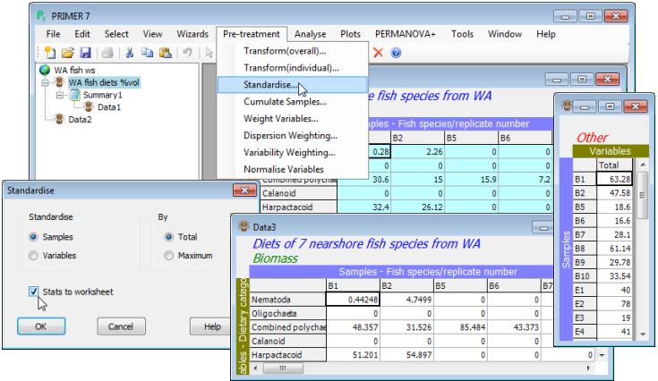
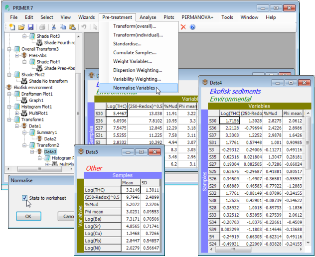
Stats to worksheet
Several of the routines in PRIMER 7 also incorporate a check box for sending summary statistics used in that routine to a further worksheet. Here, this results in a second sheet (probably named Data4), which is just a single column of totals across prey species for each of the gut samples. This is the same data as previously obtained with Analyse>Summary Stats>(For•Samples) & (✓Sum), in Section 3. (There is often more than one way of obtaining the same information in PRIMER!). Another example of summary statistics being sent to a separate worksheet is for the Normalise pre-treatment option – see below – for which the mean and standard deviation of each variable, used in the normalisation process, can be sent to a separate sheet. If this option is not selected, the same information is usually sent to a text-format results window, which can be viewed from the Explorer tree but cannot be further manipulated (unless then saved as an external .txt or .rtf file and edited in a text editor – or directly copied and pasted into Excel column(s) – to re-input as a new sheet).
Standardising species
Pre-treatment>Standardise can also be used to standardise the matrix on the variables axis, e.g. to ensure that each species is given equal weight in any ensuing similarity calculation by making their totals across samples all add to 100, with (Standardise•Variables) & (By•Total). There is an alternative option, (By•Maximum), to scale each species so that its maximum value across samples is always 100. Similar species standardisations are already built into some resemblance measures, e.g. the Gower coefficient $S_{15}$ (see Section 5) scales all species to have the same maximum, in effect, because it divides each variable through by its range (and for most species the minimum value across all samples is usually 0). For analysis of community samples, however, such species standardisation (by totals or maxima) is usually undesirable because it gives rare and very low abundance species as much weight (usually more weight in practice) than common and abundant ones. Variable standardisation, over samples, occasionally has a role with non-assemblage data which is still in the form of positive ‘quantities’, taking values down to zero but on non-comparable scales. Generally more useful though, for environmental-type matrices (where measurement scales differ, zero may play no special role at all, and values can be negative, especially after transformation) is what PRIMER refers to as normalisation – removing both scale and location differences amongst the variables (see below). The major use of variable standardisation is for the multivariate analysis of species rather than samples. To avoid the problems of standardising rare species, this first requires reduction to the ‘most important’ species, using the techniques of the last section. Then species standardisation is an important step in determining groups of species that display a coherent response across the set of samples; see Section 10 and Chapter 7 of the CiMC manual. File>Save Workspace the current form of the WA fish ws, for further use later, and close it.
Transforming (overall)
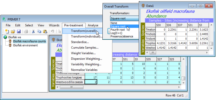
Transformation is usually applied to all the entries in an assemblage matrix of counts, biomass, % area cover etc., in order to downweight the contributions of quantitatively dominant species to the similarities calculated between samples (see Chapters 2 and 9 of CiMC). This is important for the most commonly-used resemblance measures like Bray-Curtis similarity, which do not incorporate any scaling of each species by its total or maximum across all samples. The more severe the initial transformation, the more notice is taken of the less-abundant species in the matrix. It is for the user to choose a balance between contributions of dominant and less abundant species, in the specific context, by picking from the sequence: None, Square root, Fourth root, Log(X+1) and Presence/ absence. (Reduction to presence/absence, i.e. 1/0, is thought of as a transformation since it would be the logical end-point of taking ever more severe power transforms: square root, 4th root, 8th root, …, and it is clearly one way in which less abundant species are given a similar weight to abundant ones.) If standardisation of samples by total is also required, for example to ameliorate the effects of differing sample volumes, it is logical to standardise first, then transform.
Open the previously saved workspace Ekofisk ws from the C:\Examples v7\Ekofisk macrofauna directory (or open Ekofisk macrofauna counts.pri and Ekofisk environmental.xls into a clear workspace, Section 1). Edit>Properties on the count matrix shows that 173 species were found across the 39 sites, which are ordered in increasing distance away from the oil-field centre (the putative source of a pollution gradient, diluting with distance). It is crucial to stress at this point that an initial reduction in the number of species entered into the later multivariate analyses of these samples is not required - as just remarked, it is the job of the transformation and the similarity measure to balance contributions from abundant and rarer species. However, purely in order to visualise the effect of the differing transformations, on a more manageable number of species, take Select>Variables>(•Use those that contribute at least 2 %), which selects 46 ‘most important’ species (you can see that is it 46 by clicking in the last row of the selected array, when the row and column position of the cursor will be seen at the bottom right of the PRIMER desktop). On this reduced matrix, take Pre-treatment>Transform (overall)>(Transformation:Square root), and also the options for Fourth root and Presence/absence. Rename the four ‘Datan’ sheets appropriately, e.g. by clicking twice (slowly) on their name in the Explorer tree and typing in Square root etc.
Shade plots to aid choice of transform
A major new feature in PRIMER 7 is the large number of additional plotting routines, one of the conceptually simplest but most powerful being Shade Plots, which are simple visualisations of the data matrix, with darker (or different colour) shades in each cell of the array representing higher abundances. White space denotes the absence of that species (row) in that sample (column) and full black the maximum abundance (or biomass etc.) in the array. Grey (or one/two colour) shades are linearly proportional to the intermediate abundances, as shown in a shade/colour key. Clarke KR, Tweedley JR, Valesini FJ 2014, J Mar Biol Assoc UK 94: 1-16 demonstrate the usefulness of shade plots in getting a ‘feel’ for a sensible choice of transformation for the context, e.g. if an assemblage analysis needs to take account of a wide range of common and less abundant species but the current shade plot is largely a sea of white space – because at the current transformation most abundances are still dwarfed by those for the dominant species – then the need for a heavier transformation is immediately seen. At the opposite extreme, if most of the cells from species which are present are displayed at about the same (dark) intensity then the data is likely to have been overtransformed into, effectively, presence or absence, and this may not be the required quantitative analysis.
On both the original and transformed Ekofisk macrofauna sheets take Plots>Shade Plot, to give:
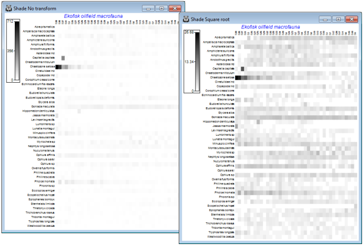
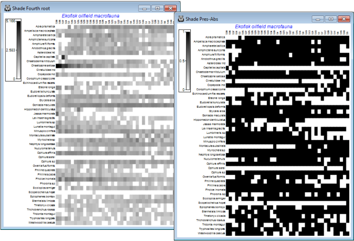
The choice looks to be between square root and fourth root, but note how the fourth-root matrix largely reflects the P/A structure, with the quantitative information little used. And after restoration of the 125 species (<2% of the composition anywhere and temporarily eliminated, purely for clarity of the plots here), they are also likely to add a great deal of random ‘noise’ on this scale. At the other extreme, the previous page shows that a failure to transform at all would leave a multivariate analysis (based on a measure such as Bray-Curtis) dependent only on a small handful of dominant species. Be aware of the dangers of ‘choosing the transformation which gives you the answer you want!’ but these plots suggest that the (relatively mild) square root transform might be relevant for data of this type (macrobenthic studies around N Sea oil-fields) – allowing the abundant species to play a greater role, but also taking into account contributions from a wide range of less-dominant species. Whether a multivariate analysis can discern any pattern of change with distance from the oil-field is more open to question, on the basis of this plot! The sites (x axis) are ordered from left to right in increasing distance from the oil-field but a matching trend in assemblage pattern is quite hard to discern (but is clearly present – see Section 8). We shall see later that astute re-ordering of the y axis (species) is visually helpful here (though a multivariate analysis ignores the ordering of variables!), and can be accessed from the Graph>Special>Re-order menu. Discussion of the wide range of possibilities on this dialog is deferred until Section 10, under Wizard>Matrix display.
Transforming abiotic variables
Transformations may be appropriate for environmental variables too, though usually for a different reason (e.g. in order to justify using Euclidean distance as a dissimilarity measure on normalised variables). However, these are usually selective transformations, required only for some variables, and with different transforms potentially applicable to variables of different types. The global Pre-treatment>Transform (overall) applies the same simple power or log transform to all variables, whereas Pre-treatment>Transform (individual) operates only on highlighted portions (usually sets of variables), and can allow user-defined expressions if a specific formula is appropriate to a certain variable. More sophisticated data manipulations with user-defined expressions are deferred to Section 11; here we concentrate on one or two commonly used transforms for abiotic variables.
In the Ekofisk ws, the Ekofisk environmental sheet holds 9 variables measured on sediments at the same set of 39 sites: total hydrocarbons (THC), several heavy metals, redox and two particle size measures, % mud and $\phi$ mean. The first variable in the sheet is just distance in km from the oil-field centre, not of itself a measure which organisms in the assemblage will respond to, and which should not be used for any assessment of the pattern of environmental change around the field.
Draftsman, histogram & multi-plots
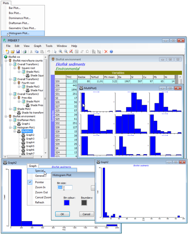
Temporarily deselect the Distance (as in Section 3), and run Plots>Draftsman Plot on the other 9 variables; also Plots>Histogram Plot (a new plotting feature in PRIMER 7). The latter leads to an example of another new feature, a Multi-plot (see Section 7), in which the window is divided into row and column cells (the numbers of which are under user control), each of which contains a standard graphics window. The multi-plot can hold graphs of different types (e.g. a multi-plot which will often be met mixes MDS ordinations and their associated Shepard diagrams, Section 8) but typically all component plots are of the same type, as here when they hold histograms for each of the 9 variables. Clicking on a cell of the multi-plot will cause that component plot to be shown at normal size and able to be operated on, in terms of changing axis labelling, titles etc. These general editing operations for plots are covered in Section 6, but each plotting routine has some specialised operations that apply only to that plot type and the one that might be of use here is to change the histogram bin width, e.g. for the THC histogram take Graph>Special>(Bin size:50). To shut down the full version of the component plot simply close it with  and click on a further component.
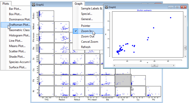
The Draftsman plot is simply a set of pairwise scatter plots of all 36 combinations of the 9 variables laid out in a single lower triangular graph array (this is not a multi-plot note, though individual portions of the plot – down to single scatter plots – can be viewed by zooming into the plot, a general feature available with all graphics through the  icon or the Graph menu, Section 6). Whilst histograms would often be used to look at the distribution of individual variables over the samples, the scatter plots of the draftsman plot can be an equally effective way of viewing this, especially if there are too few samples to bin into a meaningful histogram.
Transforming (individual)
Both the Draftsman and Histogram Plots show that several of the Ekofisk abiotic variables are highly right-skewed (tail to the right), and it would be wise, if we are to limit the distorting effects of outliers and normalise the data to a desired common measurement scale, to subject THC and the heavy metal concentrations to a strong transformation such as log(x). The particle size variables do not need further transformation ($\phi$ mean is already on a log scale). There is a case for regarding Redox as left skewed (it certainly has a large negative outlier), so we shall take the opportunity to demonstrate how to achieve a (mild) reverse power transform: $(a – x)^b$.
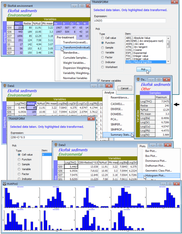
Highlight the THC, Ba, Sr, Cu, Pb, Ni variables and take Pre-treatment>Transform (individual). The transform operation itself can be any of the Transform(overall) options: square root, fourth root, log, reduction to pres/abs, using the Expressions: Sqr(V), V^0.25 ($\equiv$ Sqr(sqr(V)), log(1+V), PA(V) respectively, in which V (value) stands for any highlighted data entry (note that upper or lower case is not important in the expressions). But it is not limited to these: many other transforms can be constructed. In fact any expression using the Basic language syntax is permitted, involving operators: +, -, * (times), / (divide), ^ (power); functions: Sqr, Log (to base e) etc. as above, and Abs (absolute value), Atn (arctan), Exp (exponential), Int (integer part of a number) and many others; and even logical operators: =, <, >, <=, >=, which return –1 if true, 0 if false. (An example of the latter might be to draw attention to cells with large counts using an expression like V>1000). For a comprehensive list of expression options take Help on the Transform dialog box and click on Transform expression. Operations can extend still further, to generate new entries as combinations of samples or variables (and even factors or indicators or other worksheets), but examples of these are deferred until Section 11. In this case you simply need the Expression: log(V) which you can type directly into the Expression box or select the function from the Pick box: (Type•Function) & (Item: Log(.) Natural logarithm)>Pick. The action of the Pick button is to place the selected function around the default entry already in the Expression box (of just V). Check the expression is the one you intended and OK, to obtain a new sheet in which the concentration variables have been log transformed – their labels indicate this if you have left on the default of (✓Rename variables).
Note that the remaining variables have also been carried across to the new sheet but untransformed. This is the result of only highlighting the requisite variables rather than fully selecting them, with Select>Highlighted. (Had you done the latter then only the transformed variables would have been carried across to the new sheet, and you would have had to Select the others from the original sheet and Tools>Merge(d) them with the new, transformed variables). Now highlight the single Redox variable on the new sheet and Pre-treatment>Transform(individual)>(Expression: (250-V)^0.5). This reverses the distribution around a value just larger than its maximum, turning a mildly left-skewed shape into a mildly right-skewed one, and then the square root transformation will tend to remove that (mild) right-skewness – stronger would be to use log(250-V). Finding the maximum value for a variable is now easy with Analyse>Summary Stats>(For•Variables) & (✓Maximum). Again a new sheet is produced with the required mix of log, reverse square root and no transforms on different variables, and the efficacy of these in reducing the effects of outliers can be seen by another set of Plots>Draftsman Plot or Plots>Histogram Plot.
Normalising variables
It is typical of a suite of physico-chemical variables (or biomarkers, water-quality indices etc.) that they are not on comparable measurement scales, unlike assemblage abundances. All multivariate analysis methods are based on resemblances between samples that add up contributions across the variables. This make no sense if there is not a common scale (transformation does not help in this regard). If the similarity or distance coefficient does not have some form of internal adjustment to put variables onto a common scale (the commonly used Euclidean or Manhattan distance measures do not), then it is important to pre-treat the data to achieve this. The standard means of doing so is normalising. Literature terminology is inconsistent here, but what PRIMER means by normalising is that from each entry of a single variable we subtract the mean (across all samples) and divide by the standard deviation of that variable. This is carried out separately for each variable. It is simply a scale and location change, and does not change the shape of the histograms above, for example. It does not therefore ‘convert the variable to normality’ – this is essentially what the transformation is trying (approximately) to achieve – but it makes the mean 0 and standard deviation 1, so that all variables now take values over roughly the same limits: typically (for a normal distribution) the range –2 to +2 covers roughly 95% of the entries, making contributions to (say) Euclidean distance from different variables comparable, and effectively giving each variable the same weight. This process is sometimes known, especially in the statistical literature, as standardisation, but PRIMER reserves the term standardise for scaling positive quantities only, by dividing by their total or maximum. Standardisation would therefore not succeed in putting onto a common scale variables for which zero is not a meaningful (and attained) end point of the scale, as is true for of many abiotic variables, such as temperature. And in a marine context, salinities may fluctuate over a narrow – but still potentially important – range well away from zero; standardisation (of variables) would then be completely ineffective. Note that, unlike standardising, normalising only makes sense – and is therefore only offered – for variables, not for samples.
On the transformed environmental variable matrix from the previous page, take Pre-treatment> Normalise variables>(✓Stats to worksheet), and note how the resulting variables now take values over comparable ranges, roughly –2 to +2. They are now ready for entry to Analyse>Resemblance>(Measure•Euclidean distance), using the methods of Section 5. Save Ekofisk wk.
Dispersion weighting of species
When variables are on different measurement scales, there is little viable alternative to normalising each variable (as above) thus equalising, in effect, their contributions to the multivariate analysis. When variables are (ostensibly) on the same scale, e.g. species abundances, then their respective contributions to commonly-used similarity coefficients, such as Bray-Curtis, will differ, based on the relative magnitude of counts (or transformed counts). Larger abundances are always given more weight (unless ‘transformed out’ to purely presence/absence). This may not always be desirable, however. For example, some numerically dominant species may give highly erratic counts over replicate samples within a site (or time or condition), perhaps due to an innately high degree of spatial clumping of individuals (individuals of that species arrive in the sample in clusters). This is likely to add ‘noise’ rather than ‘signal’ to the multivariate analysis, and downweighting of such species is called for, in relation to other species which are not spatially clustered, but have the lower variance associated with Poisson counts (the individuals arrive in the sample independently of each other). The weighting is achieved by the Pre-treatment>Dispersion weighting procedure, (Clarke KR, Chapman MG, Somerfield PJ, Needham HR, 2006, Mar Ecol Prog Ser 320: 11-27), covered in detail in Chapter 9 of the CiMC manual.
The differential downweighting is carried out by dividing the counts for each species by their index of dispersion $\overline{D}$ (variance to mean ratio, a ‘clumping’ measure), calculated from replicates within a group (site/time/treatment etc.), and then averaged across groups. The weighting is valid under rather general conditions, not unrealistic, but the original derivation did require: a) data to be real species counts, not densities standardised to some unit volume or substrate area; b) independent replicates within each of a set of sample groups, so that there is a basis for assessing within-group variance structure; and c) those replicates to be of a uniform size (strictly ‘quantitative sampling’). Downweighting is only applied where a species shows significant evidence of clumping, this being tested by an exact permutation test, valid for the very small counts that are typical of many species. The resulting dispersion-weighted matrix has a common (Poisson-like) variance structure across species but unchanged relative responses of species in different groups. This is an important point: there is no attempt here to place greater emphasis on those species which best show up a given group structure (e.g. best separate control from polluted conditions). Such ‘constrained’ methods run the risk of circular arguments: selecting out only those species that tell you the answer you wanted in the first place! All that dispersion weighting does is divide through each row of the matrix (species) by a constant, so that a different balance of species contributions will be obtained by the subsequent analysis. These weights are calculated solely using information from replicates within each group, not across groups, so a consistent species (low variance-to-mean ratio within groups) will be given a high relative weight even if it shows no difference at all between groups.
If dispersion weighing of a count matrix is contemplated, this pre-treatment step must be carried out before any transformation. It may still make sense then to transform the dispersion weighted data sheet: a species which has large mean abundance at some sites, and is found in very consistent numbers in all replicates from those sites, will still tend to dominate the similarities. Transforming now has the strict objective of balancing contributions of consistent abundant species with equally consistent but less numerous species. Previously, it was really used for this purpose and to reduce the impact of large but erratic counts of some species – but the latter can now be catered for by dispersion weighting. Whilst this will eliminate the need for transformation in some cases, it will still be required in others (Clarke KR, Tweedley JR, Valesini FJ 2014, J Mar Biol Ass UK 94: 1-16), to down-weight large counts which are also consistent. (The example there is of counts of small-bodied fish species, and demonstrates the usefulness of shade plots – seen earlier in this section – in determining whether/what transform may be needed after dispersion weighting.)
Chapter 9 of CiMC also discusses generalising the dispersion weighting concept to data which are not strict counts, but are density, area cover or biomass, etc. For ‘quantity’ data of this type, on a common measurement scale, it can still make sense to apply dispersion weighting, e.g. colonial species in large patches can have high variability for their mean area, over replicate quadrats (as measured by grid intersections, perhaps), and thus less inherent reliability than individual small-bodied, motile species with the same mean area cover. However, a dispersion index of 1 no longer has meaning (values depend on the measurement units) and permutation testing of $\overline{D} = 1$ thus also makes no sense. The PRIMER 7 dialog for Pre-treatment>Dispersion Weighting now gives a tick box not to perform this test, and division of entries by $\overline{D}$ then takes place whatever its value.
(Fal estuary copepods)
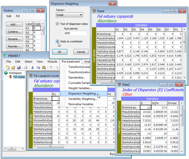
Sediment copepod assemblages (and other fauna) from five creeks of the Fal estuary, SW England, were analysed by Somerfield PJ, Gee JM, Warwick RM 1994, Mar Ecol Prog Ser 105: 79-88. The sediments of this estuary are characterised by high and varying concentrations of heavy metals, a result of tin and copper mining over hundreds of years. The copepod data consist of 23 species found in 27 samples, consisting of 5 replicate cores spanning each creek (Mylor: M1-M5; Pill: P1-P5; St Just: J1-J5; Percuil: E1-E5; and 7 from the largest creek, Restronguet: R1-R7). These are in directory C:\Examples v7\Fal benthic fauna, worksheet Fal copepod counts(.pri), with a factor Creek identifying samples from the 5 creeks. There are also environmental cores (of silt/clay ratios, heavy metals etc.) matching these 27 sample locations, held in an Excel file Fal environment(.xls), plus nematode densities, macrofaunal counts and biomass, and associated aggregation files.
File>Open the copepod data and take Pre-treatment>Dispersion weighting>(Factor: Creek) & (✓Test of dispersion index) & (Num perms: 1000) & (✓Stats to worksheet). The Data1 sheet gives the dispersion weighted counts, which are either ready to go into the Analyse>Resemblance step of the next section, or could be mildly transformed before they do so, as shown earlier with Pre-treatment>Transform(overall)>(Transformation: Square root). There seems little need for the latter, however, since the dispersion weighting has already succeeded in downweighting the larger, erratic counts coming from P. littoralis, R. celtica, E. gariene and T. discipes and the somewhat less erratic P. curticorne and M. falla – the matrix Data1 now has no dispersion-weighted ‘counts’ in double figures, and the subsequent untransformed analysis will not be dominated by a small set of species. In three columns, Data2 gives: the mean dispersion indices $\overline{D}$ for each species; the evidence for clumping (i.e. the % significance level for a test of $\overline{D} = 1$); and the actual divisor used for that species row, which is 1 if the test does not reject this hypothesis at 5% (or better). Thus, T. discipes values are divided by 13.67 but Brianola sp. remains unchanged, though $\overline{D} = 1.5$. You might now like to run the routine again for the Fal nematode abundance file, which inspection shows must be numbers scaled up to a density, not real counts (e.g. there are no entries of 1!). The tick box for the test must be unchecked, the resulting $\overline{D}$ values are all >>1, but weighting by $\overline{D}$ is still justifiable.
Other variable weighting
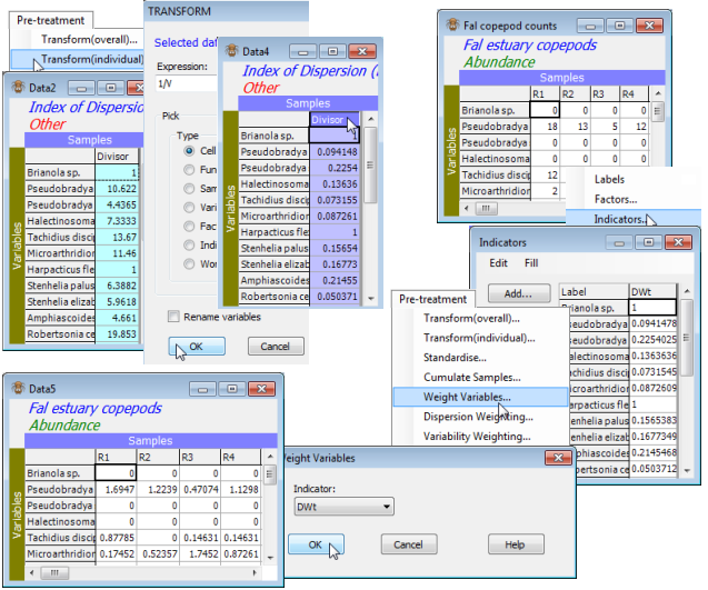
There are other cases in which variables (species) might need prior weighting, e.g. when a species is known to be often misidentified, its contribution (and those of the species it is mistaken for) can be reduced by multiplying the entries in the two species through by some downweighting constant. This is achieved by placing weights for each species in an Indicator (see Section 2) and taking Pre-treatment>Weight variables, supplying the indicator name. In this context, most weights would be 1, with a value less than 1 used for downweighting less-reliably identified species (the default weight could be 100, or any number, since similarities such as Bray-Curtis are invariant to a scale change). A further context in which this routine might be useful is to convert counts to approximate biomass, using a known average weight of an individual of each species. Also dispersion weighting is seen just to be another case of variable weighting, with weights as the reciprocal of the Divisor column. You might like to demonstrate this for the Fal copepod counts example above, by selecting or highlighting the Divisor column from Data2 then take Pre-treatment>Transform(individual)> (Expression:1/V), highlighting the new column and copying (Ctrl-C) to the clipboard; opening Fal copepod counts, Edit>Indicators>Add>(Add indicator named:DWt), highlighting that blank new column and pasting (Ctrl-V); and finally Pre-treatment>Weight Variables>(Indicator:DWt). The resulting matrix should be identical to Data1. Save the workspace as Fal ws for later use.
Mixed data types
Another example might be in attempting to reconcile two different types of data in the same matrix, e.g. counts of motile organisms and area cover of colonial species. These cases can be problematic. One solution is to use a similarity measure such as the Gower coefficient, which scales the range of each species across samples to be identical, but this generally performs badly because very rare species are given the same weight as very common ones. A preferable alternative is to use Bray-Curtis similarity as usual, but prior to that Weight Variables to convert counts into approximate area cover, species by species, or both counts and area cover into a rough estimate of biomass, or even just to balance the two sets of variables against each other in some arbitrary way, e.g. give the cover numbers 10 times as much weight, or 10 times less weight, keeping the counts unchanged, and see what difference it makes to the analysis. (See also the discussion on p5-19 of CiMC.)
Variability weighting
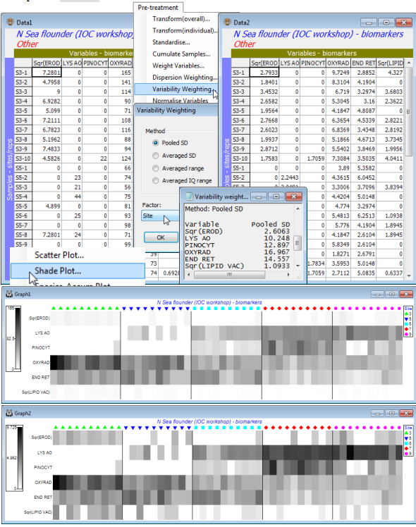
Pre-treatment>Variability Weighting is a new option in PRIMER 7, which bears similarities to the idea of Dispersion Weighting. This was introduced by Hallett CS, Valesini FJ, Clarke KR 2012, Ecol Indicat 19: 240-252 in a context where the variables were ‘health indices’ of fish communities and is exemplified here in a comparable case of a ‘biomarker’ suite, measured on individual fish, from locations with putatively differing contaminant impacts. Such indices typically behave more like environmental-type variables, with differing measurement scales and without the presence/ absence structure of community matrices, so that transformation, normalisation and then a distance resemblance measure (e.g. Euclidean) would be appropriate (see earlier this section). The downside of normalising is, however, that all variables are essentially given equal weight in that calculation – but how else can one sum variable contributions over different units other than to shrink or stretch their scales to a common ‘spread’ (SD of 1)? (The location shift involved in normalising is actually irrelevant as far as distance measures such as Euclidean or Manhattan are concerned, because they are a function only of differences between sample values for each variable, so a subtracted constant disappears – the key thing is only the scale change to each variable). One possible answer is to scale each variable to a common spread (e.g. SD of 1) of its replicates within groups, not the full set of values across the groups (where the groups are the combinations of site, time etc.). As with Dispersion Weighting, the idea is that some indices may be inherently less reliable than others, with erratic values for genuinely independent replicate observations within groups, so that it is desirable to give more weight to variables with lower (average) replicate variability. The variables now, though, are no longer ‘quantities’ – indeed after some transformations (e.g. log) they may take negative values, the mean may even be zero and dividing by the Index of Dispersion (ratio of variance to mean) will make no sense. Instead, the Variability Weighting dialog offers a range of possible rescalings of replicates, by: •Pooled SD (as would be calculated from 1-way ANOVA, by square-rooting the residual variance estimate, the logically best option for normally distributed variables with common replicate variance across groups); •Averaged SD (a simple mean of SDs computed separately for each group); •Averaged range (mean of the separate ranges – if used with Manhattan distance this is a more subtle version of the Gower coefficient, see Section 5); and •Averaged IQ range (mean of the inter-quartile ranges for each group, potentially a more relevant spread measure than SD for non-normally distributed – but continuous – replicate observations). As with Dispersion Weighting, all samples for each variable are simply divided through by their own averaged replicate ‘spread’, a new sheet formed and the divisors given in a Results window.
(Biomarkers for N Sea flounder)
The directory C:\Examples v7\N Sea biomarkers holds a data sheet N Sea flounder biomarkers(.pri) of biochemical and histological biomarkers measured concurrently on flounder caught at 5 North Sea sites (labelled S3, S5, S6, S7 and S9), running on a putative contaminant gradient from the mouth of the Elbe (S3) to the Dogger Bank (S9). It is a multivariate study because all variables were measured on each of 50 (pools of) fish, consisting of 10 sample pools from each site. This was part of a larger practical workshop on assessing ‘biological effects’ techniques for detecting pollution in the marine environment – the IOC Bremerhaven workshop (Stebbing ARD, Dethlefsen V, Carr M (eds) 1992, Mar Ecol Prog Ser 91, special issue). The 11 biochemical and sub-cellular variables measured: EROD, lysosomal acridine orange (LYS AO), lysosomal neutral-red retention (LYS NRR), pinocytosis (PINOCYT), oxyradicals (OXYRAD), endoplasmic reticulum (END RET), N-ras, ubiquitin, cathepsin D (CATH D), tubulin and lipid vacuoles (LIPID VAC), which are a mixture of continuous, heavily discretised and (one) presence/absence variables.
Open the N Sea flounder biomarkers sheet; note this time the 11 variables are columns and the 50 samples the rows, with a defined Site factor. Highlight, then select, only the 6 continuous variables EROD, LYS AO, PINOCYT, OXYRAD, END RET and LIPID VAC. They are all statistically well-behaved variables without strong outliers though the replicates for EROD and LIPID VAC are somewhat right-skewed, so it might be beneficial to highlight these two and take Pre-treatment> Transform(Individual)>(Expression:Sqr(V)) for a mild square root transform of those variables. *Pre-treatment>Variability Weighting>(•Pooled SD) & (Factor:Site) then results in a sheet in which the columns (variables) are just divided by the pooled SD values given in the results window ( Variability weighting1). The Data2 sheet is now ready to go into the Analyse>Resemblance> (Measure•Euclidean distance) routine of the next section. (Note that, though the Pooled SD divisor is really designed for continuous data, nothing goes dramatically wrong by leaving all 11 variables in the computations, though the discrete variables need to be at least ordered categories, as here).
Finally, the effect on the relative contributions of each of the 6 variables to the Resemblance calculations, before and after the Variability Weighting, can be neatly seen by submitting both Data1 and Data2 to Plots>Shade Plot. The (transformed) EROD and Lipid variables would clearly be largely ignored without the rescaling but, less trivially, the variable clearly given greater weight (darker shading) by the rescaling is LYS AO, seen to have consistently high or consistently low values for replicates from the same site, in the original plot. The plots have been slightly modified, simply to accentuate the site differences on the x axis, using the extensive menu choices, e.g. for labels and adding symbols, Graph>Sample Labels & Symbols>(Symbols:(✓Plot) & (✓By factor) & Site) and taking off the tick box for Labels. This is a generic menu that covers many types of plot and will be seen again in Section 6 and beyond. Also, there are Special menus applying only to individual types of plot and one of those is demonstrated by the dividing lines between sites, which are produced by Graph>Special>Reorder>(Samples:Constraint•Factor groups:Site). The many other options on this Special menu for the shade plot routine are discussed in Section 10. Save the workspace as N Sea ws.
Cumulating samples
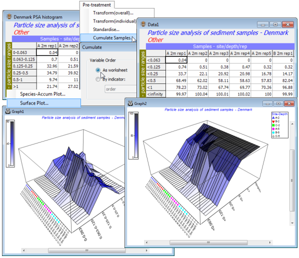
The remaining option on the Pre-treatment menu is Cumulate samples, which successively adds up the entries across variables, separately for each sample. It is only appropriate when all variables share a common measurement scale, and when the order in which they are listed is meaningful; it is thus not relevant standard species-by-samples data. It may be useful in analysing arrays in which variables are different body-size categories of a single species, or different particle sizes classes in Particle Size Analysis (PSA) etc, and entries are the frequencies or quantities of each size class in each sample (see CiMC, Chapter 8). Such data is typically analysed by univariate methods, fitting parametric particle-size distributions and comparing parameter estimates over samples. That can be problematic: histograms do not fit the models, summary statistics like mean and variance do not capture features such as bimodality, tests are incorrect because the data are not real frequencies, it is difficult to synthesise many such samples etc. This can be side-stepped by multivariate analysis, defining the similarity of pairs of size-class distributions. To take into account ordering of the sizes, when histograms are not smooth, it may sometimes be preferable to compare pairs of cumulative distributions (sample distribution functions) rather than the histograms (sample density functions).
(Particle sizes for Danish sediments)
Sediment particle size data from 6 size ranges at 3 sites (A, B, C), at 2 depths (2m and 5m), and 5 replicate samples from each site/depth combination are in C:\Examples v7\Denmark PSA\ Denmark PSA histogram. The data are already standardised to % composition – if not, you would need Pre-treatment>Standardise>(Standardise•Samples)&(By•Total). So, take Pre-treatment>Cumulate Samples>(Variable Order•As worksheet). The variable labels are now inaccurate, so replace them by copying/pasting cumulative from Edit>Indicators and into the Edit>Labels>Variables dialog.
Surface plots
The smoothing effect can best be seen by Plots>Surface Plot of both Data1 and Data2 sheets – a further graph type new to PRIMER 7, but which should be reserved only for cases such as this, where there is genuine ordering of the variables. Symbols can be added to the sample axis with Graph>Sample Labels & Symbols, and colour shading introduced (as it could have been with the above Shade Plots) by Graph>Special>Key. Save the workspace as Denmark ws for use later.