5. Resemblance: similarities, dissimilarities and distances
- Resemblance matrices
- Standard resemblance choices
- Bray-Curtis similarity
- Zero-adjusted Bray-Curtis
- (Tikus Island coral cover)
- Euclidean distances
- Index of Association
- Accessing other resemblance measures
- Distance measures
- ‘Modified Gower’
- Similarity to dissimilarity
- Quantitative similarity measures
- Presence/ Absence similarities
- Quantitative measures on P/A data; Unravelling resemblances; Scatter plots
- Other coefficients
- Between-curve distances
- (Plymouth particle-size analysis)
- Taxonomic distinctness/ aggregation files
- Taxonomic dissimilarity measures
- (Groundfish of European shelf waters)
- Relatedness supplied as resemblances
- Analysing between variables
- Correlation between variables
- Correlation as similarity
- Corrections for missing data
- Saving & opening triangular matrices
Resemblance matrices
Fundamental to the operation of PRIMER and (explicitly or implicitly) any fully multivariate analysis, is an appropriate definition of resemblance between every pair of samples, based on whether the suite of recorded variables (species, environmental variables, biomarkers, particle-size classes or whatever) take similar or dissimilar values. What is meant by ‘similar’ is a function of the context and purpose of the analysis, and PRIMER 7 gives nearly 50 definitions to choose from (many are covered by the general reference work Legendre P & Legendre L 2012, Numerical ecology, 3rd English ed, Elsevier, called L&L from now on). Within PRIMER, similarity is taken to range over 0 to 100 (perfect similarity), dissimilarity is the complement (100 – similarity), whereas distance ranges from 0 to infinity. PRIMER 7 uses the term Resemblance to cover all three concepts: •Similarity, •Dissimilarity or •Distance, and also a number of specialised coefficient types which are useful to distinguish separately: •Distance$^2$; •Correlation (which is defined over the range –1 to 1 and is therefore not directly a similarity, though it may be transformed into one in at least two different ways – see the Transform option in Section 11); •R (the pairwise ANOSIM R statistic – see Section 9); and •Rank (where similarities or dissimilarities are turned into ranks, i.e. the positive integers, with averaged values for any tied ranks – which can be used directly as a distance matrix. The unifying structure here is that these are all pairwise coefficients and they are all symmetric (the resemblance of samples 1 and 2 is the same as that of 2 and 1), so resemblances between every pair of samples form a lower triangular matrix, with no diagonal. They are displayed with the upper triangle absent and the specific Type as the second heading in the sheet window, so it should always be clear when the active window is a resemblance matrix and when it is a data sheet. (This matters because the available menu options change with the active window type).
Standard resemblance choices
A detailed discussion of the competing properties of different resemblance matrices is outside this manual’s scope (see L&L, CiMC Chapters 2 & 16, or Clarke KR, Somerfield PJ, Chapman MG 2006, J Exp Mar Biol Ecol 330: 55-80). Novice users are recommended to take one of the main options (the defaults): Bray-Curtis similarity for biological assemblage data; Euclidean distance (having first normalised) for physico-chemical, biomarker or morphometric data etc., in which variables are not on comparable ranges or the same measurement scale at all; and (non-normalised) Euclidean distance for body- and particle-size histograms (first standardised), growth curves etc.
Bray-Curtis similarity
The most commonly-used similarity coefficient for biological community analysis, because it obeys many of the ‘natural’ biological guidelines in a way that most other coefficients do not (see CiMC), is the Bray-Curtis similarity, defined between samples 1 and 2 as:
$$S _ {17} = 100 \left[ 1 - \frac{\sum_{i} | y_{i1} - y_{i2} | }{\sum_{i} y_{i1} + \sum_{i} y_{i2} } \right] \equiv 100 \frac{ \sum_i \min \left( y_{i1}, y_{i2} \right) }{ \left( \sum_{i} y_{i1} + \sum_{i} y_{i2} \right) / 2} .$$
The two forms may not look identical but they are! Here $y_{i1}$ is the count (or biomass, % cover, …) for the ith (of p) species from sample 1, and $\sum_i$(…) denotes summation over those species. Original references to coefficient definitions are not given here (nomenclature is always a source of debate!) – see L&L, whose numbering scheme is followed where possible, hence $S_{17}$ for Bray-Curtis.
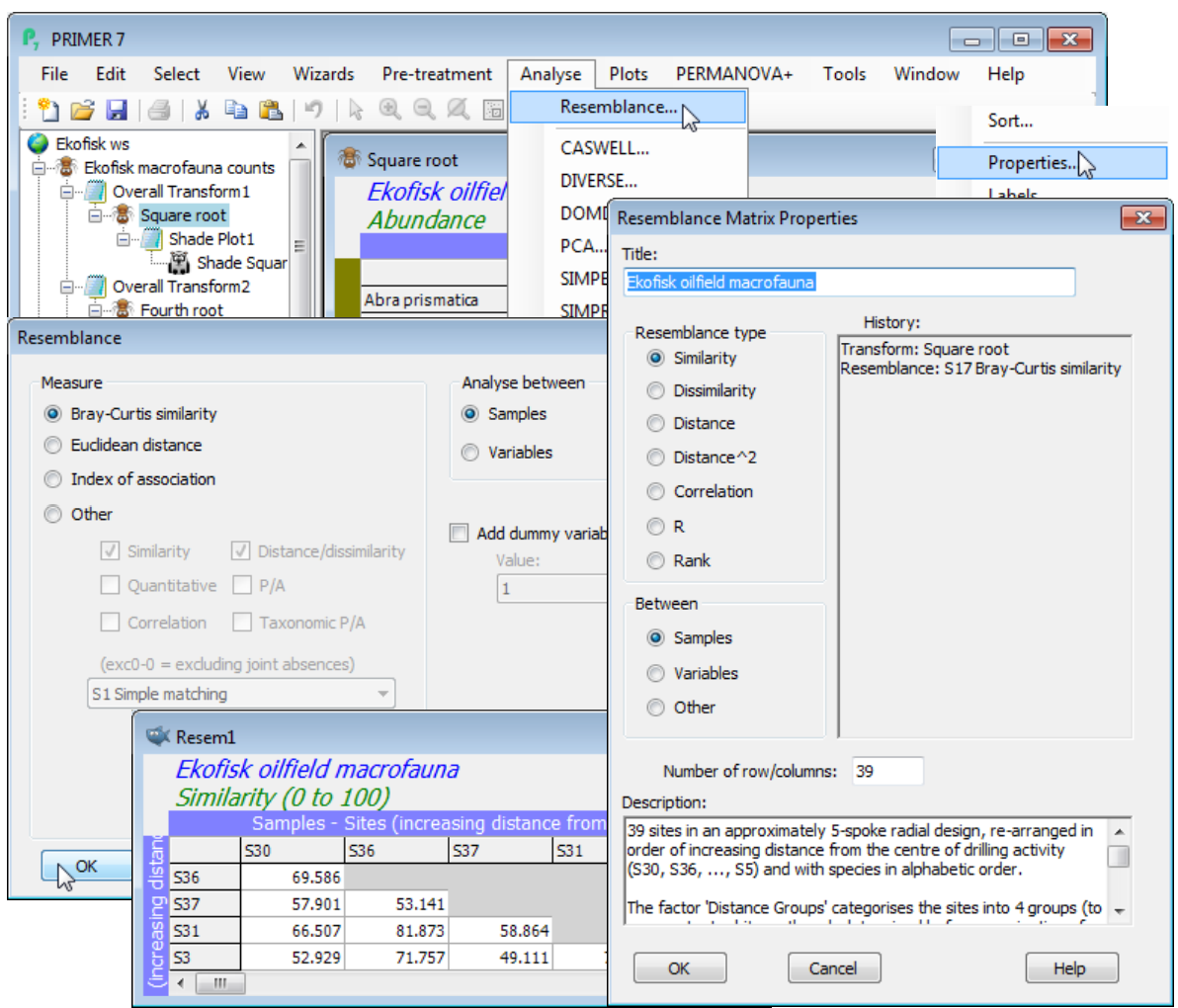
Open the workspace C:\Examples v7\Ekofisk macrofauna\Ekofisk ws from earlier, and click on the Square root counts sheet (obtained earlier with Pre-treatment>Transform(overall)>Square root). Take Analyse>Resemblance>(Measure•Bray-Curtis similarity) & (Analyse between•Samples), which are the defaults for this data type. A lower triangular matrix is produced, Resem1, which you should rename B-C on sq rt. Edit>Properties (or right-clicking over the matrix to get Properties) shows it is of Resemblance type•Similarity from 39 samples. The History box carries through the knowledge of how it was created to a subsequent Cluster or MDS ordination plot. This box is not user-editable, though the Title and Description boxes can be altered; changes to the Title are carried forward to a subsequent plot but not backward to the data sheet Square root.
Now repeat Resemblance directly on the original Ekofisk macrofauna counts, without the Pre-Treatment transformation. PRIMER tries to help – a warning message appears that no transform has been applied; community matrices usually require some transformation before calculating Bray -Curtis (though you can happily ignore this warning if you are interested in the pattern of the few most dominant species only). Cancel the calculation and resave the Ekofisk ws workspace.
Zero-adjusted Bray-Curtis
A simple modification to the Bray-Curtis coefficient adjusts its behaviour as samples become vanishingly sparse. Standard Bray-Curtis is undefined for two samples containing no species, and can fluctuate wildly for near-blank samples – two samples containing just a single individual can fluctuate between 100% similarity if the individuals are from the same species, to 0% if they are not. The zero-adjusted Bray-Curtis coefficient (Clarke KR, Somerfield PJ, Chapman MG 2006, J Exp Mar Biol Ecol 330:55-80; also CiMC, Chapter 16) damps down this behaviour – analogously to the addition of the constant 1 in the log(1+x) transformation (to cater for x=0) – by adding +2 to the denominator of the ratio in $S_{17}$. A simple way of viewing this is as adding a ‘dummy species’ to the matrix, taking the value 1 for all samples. This forces two samples with no content to be 100% similar (they share the dummy species) and two samples with a single real individual now have some similarity, whether that species is shared (100%) or not (50%). It is clear that once there are a modest number of individuals, in either sample, then the adjustment makes no difference. It can only come into force when the assemblage is virtually denuded, and should only be applied if it makes biological sense to regard two blank samples as 100% similar, because both are denuded from the same environmental cause. If blank samples can be present in very different treatments/ sites etc., because of small sample sizes and highly clustered spatial distributions of organisms, it is unwise to use the zero-adjustment – instead, remove the blanks and use standard Bray-Curtis.
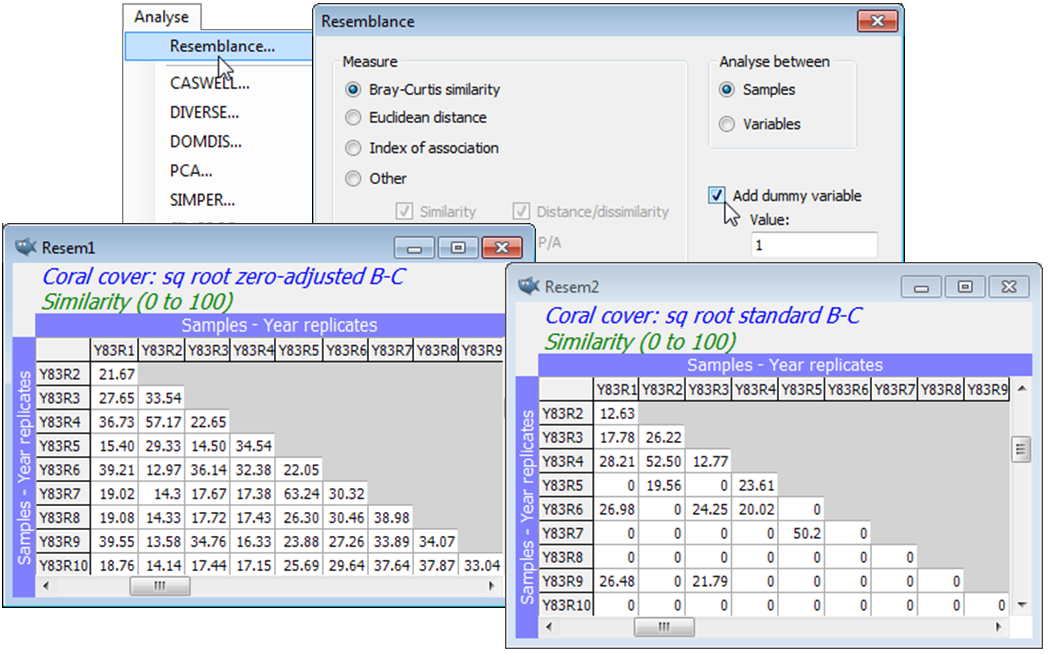
The adjustment is made by taking: (✓Add dummy variable)>(Value:1) in the Resemblance dialog. The constant 1 is appropriate to integer counts, being the lowest non-zero value attainable. This is true whether the data sheet has previously been transformed or not (the constant remains 1 under any power transform). For data on biomass, % area cover etc., the value could sensibly be chosen similarly as the lowest non-zero entry likely to be recorded (again the analogy with the log(c+x) transform is appropriate). ‘Adding a dummy variable’ can be carried out with other resemblance measures, but will only be effective for those coefficients which, like Bray-Curtis, treat joint absences of species as uninformative (e.g. Kulczynski, Czekanowski mean character difference, Canberra etc.). It is not given as an option for data type Environmental (it makes no sense then).
(Tikus Island coral cover)
Data on coral communities at a site in Tikus Island, Thousand Islands, Indonesia, over the years 1981, 83, 84, 85, 87 and 88, were reported by Warwick RM, Clarke KR, Suharsono 1990, Coral Reefs 8: 171-179. Ten replicate transects were examined each year, and the data is the length of intersection of a transect (as a percentage of transect total length) by each of the 58 coral species identified, file Tikus coral cover in directory C:\Examples v7\Tikus corals. The region was subject to a coral bleaching event in 1982 (probably El Niño related), so that the 1983 samples are very denuded of live coral – this is a classic situation in which a zero-adjusted Bray-Curtis similarity is likely to be useful, and this example is discussed in detail in the Clarke et al 2006 paper mentioned above. A dummy value of 1 is a natural choice here because the smallest non-zero entries for each species are about 1%, or marginally less. To see these entries, highlight the whole array, take say Pre-treatment>Transform(individual)>(Expression:V-10*(V=0)) and enter the resulting sheet to Analyse>Summary Stats>(For•Variables)&(✓Minimum). This works because the BASIC syntax expression computed on the value V in every cell, V-10*(V=0), returns either -1 (true) or 0 (false) for V=0, multiplies this up to -10 or 0, so when subtracted from V returns +10 in any cell which is zero and leaves non-zero values alone. Summary Stats then finds the minimum for each species. (10 in the expression could be replaced by any large number). If you run the Summary Stats again, this time (For•Samples)&(✓Minimum) you will get the lowest non-zero entry in the whole matrix.
As in the previous section, Plots>Shade Plot readily shows that a (mild) square root transform is necessary to avoid the resemblance calculation being dominated by just a couple of species with occasionally very large %cover values. So, after Pre-treatment>Transform(overall)>Square root, take Analyse>Resemblance>(Measure•Bray-Curtis similarity) & (Analyse between•Samples) & (✓Add dummy variable>Value: 1), this dummy value of 1 being equally suitable after any power transformation or reduction to presence/absence (1/0). By repeating this calculation on the square-rooted data, but without the dummy variable, a quick glance at the two resemblance matrices shows the dramatic effect of the zero-adjustment here, e.g. among the 1983 replicates. (This translates into substantial differences in the clustering, MDS ordination, ANOSIM tests etc, see Fig. 16.7, CiMC). File>Save Workspace As>(File name:Tikus ws) in the C:\Examples v7\Tikus corals directory.
Euclidean distances
Euclidean distance, an appropriate measure for environmental (and other) data types, is defined as:
$$ D_1 = \sqrt{ \sum_i \left( y _ {i1} - y_{i2} \right) ^ 2 } $$
where the $y_{i1}$ & $y_{i2}$ result from pre-treatment by transformation (sometimes) and subsequent normalisation (often). The outcome is a triangular distance matrix, which orders in the opposite direction to similarity: high similarity = low distance (= low dissimilarity). Note, however, that the user does not have to worry about which way round the resemblances are ordered: all routines will utilise the information given in the Resemblance type to make sensible choices.
Re-open the Ekofisk workspace Ekofisk ws from the \Ekofisk macrofauna directory; you should have available the transformed and normalised environmental data (Data4 perhaps) from Section 4, on which to calculate Euclidean distance. The Analyse>Resemblance dialog box now gives the default as Measure•Euclidean because Data type has been defined as Environmental, so you can take the defaults here. The result is a resemblance matrix of type Distance; the History box on the Edit>Properties dialog shows its derivation as Euclidean distance on normalised data. Compute Manhattan distance also (see next page) and rename the sheets as Euclid and Manhattan by clicking (twice, slowly) on their default Resem names in the Explorer tree. Most other measures in the lists below are not suitable for normalised environmental data but are designed for positive ‘quantities’.
Index of Association
The remaining of the three choices in the initial list, Measure•Index of Association, is essentially Whittaker’s index of association, which when calculated on samples (the default is always Analyse between•Samples)is simply just Bray-Curtis similarity on a sample-standardised matrix. [You might like to check this with the following sequences on the original Ekofisk macrofauna counts :
(i) Pre-treatment>Standardise>(Standardise•Samples)&(By•Total) then Analyse>Resemblance
>(Measure•Bray-Curtis similarity)&(Analyse between•Samples), compared with
(ii) Analyse>Resemblance>(Measure•Index of Association)&(Analyse between•Samples).]
The Index of Association is not therefore in this main list for its use on sample similarities but because it is the primary means of computing similarities among species, in their behaviour over the full set of samples. Importantly therefore, (Measure•Index of Association) almost always needs to be used with (Analyse between•Species), and the measure is then defined, over (0,100), as:
$$ IA = 100 \left[ 1 - \frac{1}{2} \sum_j \left| \frac{y_{1j} }{ \sum_{j} y_{1j}} - \frac{y_{2j}}{ \sum_{j} y_{2j}} \right| \right] $$
with 0 implying full ‘negative’ and 100 full ‘positive’ association of the two species (1 & 2 in the above equation). For its application as part of the new coherent curves method in PRIMER 7 see Section 10. Note that in PRIMER 6, the Whittaker coefficient was present only in its dissimilarity form (the $D_9$ of L&L) which is really a coefficient of dis-association since it takes larger values for samples with more differing communities. The previous nomenclature was therefore confusing and the index of association is now available in PRIMER 7 only as a similarity. Note also that all the definitions in the remainder of this section (up to the Analysing between variables box heading) are given in terms of resemblances among samples, the primary use for resemblance matrices.
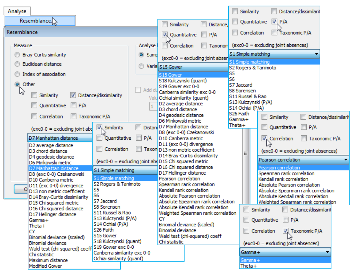
Accessing other resemblance measures
PRIMER 7 allows the user choice of 44 other resemblances, firstly divided into two (mutually exclusive) types: Similarities (including L&L’s S numbers) or Dissimilarities/Distances (including L&L’s D numbers); then most of the same coefficients split instead into Quantitative or Presence/ Absence measures; and finally two specialised groups of Correlation coefficients and Taxonomic-based P/A measures (the latter using an aggregation file of the type met in Section 2, on species relatedness). These are all accessed through the Measure•Other button and the drop-down list.
Distance measures
The distance measures defined by L&L and calculated by PRIMER 7 (in addition to $D_1$) are:
$ D_2 = \sqrt{ \frac{1}{p} \sum_i \left( y_{i1} - y_{i2} \right) ^ 2 } \text{ \hspace{25mm} average distance,} $
where the number of species p is fixed for all pairs of samples, so this is a constant multiple of Euclidean distance $D_1$ and will therefore give identical dendrograms, ordinations etc. (complete data is assumed for all these formulae, i.e. without missing values, though automatic adjustment to formulae under pairwise elimination of missing values is carried out for all measures, see later);
$ D_3 = \sqrt{ 2 \left( 1 - \frac{ \sum_i y_{i1} y_{i2} }{ \sqrt{ \sum_i y_{i1}^2 \sum_i y_{i2}^2}} \right) } \text{ \hspace{18mm} Orloci’s chord distance;} $
$ D_4 = \text{arccos} \left(1 - \frac{1}{2} D_3^2 \right) \text{ \hspace{27mm} geodesic metric;} $
$ D_6 = \left( \sum_i \left| y_{i1} - y_{i2} \right| ^r \right) ^{1/r} \text{ \hspace{26mm} Minkowski metric,} $
where r can be specified by the user (note r=1 gives Manhattan, and r=2 Euclidean distance);
$ D_7 = \sum_i \left| y_{i1} - y_{i2} \right| \text{ \hspace{34mm} Manhattan distance, }$
whose use of absolute rather than squared differences confers slightly better robustness to outliers
$ D_8 = \frac{1}{p_{12}} \sum_i \left| y_{i1} - y_{i2} \right| \text{ \hspace{25mm} Czekanowski’s mean character difference,} $
in the form where p12 is the number of species that are not jointly absent in samples 1 and 2 (the changing denominator across pairs of samples, from excluding joint absences, can make a big difference to a coefficient’s behaviour, so is indicated clearly by ‘exc0-0’ in the drop-down box).
$ D_{10} = \sum_i \frac{ \left| y_{i1} - y_{i2} \right| }{ \left( y_{i1} + y_{i2} \right) } \text{ \hspace{33mm} Canberra metric of Lance \& Williams,} $
which must exclude joint absences so that it can be defined, but is less useful than its averaged form, divided by p12, found as Canberra similarity in the quantitative similarity list;
$ D_{11} = \sqrt{ \frac{1}{p_{12}} \sum_i \left( \frac{ y_{i1} - y_{i2} }{ y_{i1} + y_{i2} } \right)^2 } \text{ \hspace{22mm} Clark’s coefficient of divergence,} $
also in the form in which double zeros are excluded from the summation and the divisor $p_{12}$;
$ D_{15} = \sqrt{ \sum_i \frac{1}{y_{i+}} \left( \frac{ y_{i1} }{\sum_i y_{i1}} - \frac{y_{i2}}{ \sum_i y_{i2} } \right)^2 } \text{ \hspace{15mm}} \chi^2 \text{(chi-squared) metric,} $
where $y_{i+} = \sum_j y_{ij}$, the sum across all samples of the entries for the $i$th species, and effectively the same, to within a constant, as the following;
$ D_{16} = \sqrt{ \sum_i \frac{1}{y_{i+}/ \sum_i y_{i+}} \left( \frac{ y_{i1} }{\sum_i y_{i1}} - \frac{y_{i2}}{ \sum_i y_{i2} } \right)^2 } \text{ \hspace{11mm}} \chi^2 \text{distance,} $
the implicit distance underlying Correspondence Analysis, which is seen to be a type of Euclidean distance, from samples which are standardised by their totals across species, and then inversely weighted by species totals across samples (the double standardisation being responsible for the practical difficulties $\chi^2$ distance can have with rare species, for which the divisor is near zero); and
$ D_{17} = \sqrt{ \sum_i \left( \sqrt{ \frac{ y_{i1} }{ \sum_i y_{i1}}} - \sqrt{ \frac{ y_{i2} }{ \sum_i y_{i2} } } \right)^2 } \text{ \hspace{5mm} Hellinger distance, advocated by Rao,}$
the only omission above being $D_{13}$, which is simply the complement of Sørensen similarity, $S_8$.
‘Modified Gower’
Anderson MJ, Ellingsen KE, McArdle BH 2006, Ecol Lett 9: 683-693 used Czekanowski’s mean character difference (above) as their preferred distance measure after a specific transformation of the original counts, advocated for its interpretable properties, namely: $y^′ = \log(y) + 1$, unless $y = 0$, when $y^′ = 0$. Choice of the base for the logarithm explicitly scales how much weight the counts get in relation to the presence/absence structure. For example, base 2 gives the step from 0 (absence) to 1 (individual) the same weight as the step from 1 to 2, or from 2 to 4, or 4 to 8 etc. Base 10 gives 0 to 1 the same weight as 1 to 10, or 10 to 100 etc. Thus high bases give more weight to the presence/ absence structure. Thus, this work mainly concerns an added transformation choice rather than a new resemblance measure, but it is convenient to bundle the transformation with Czekanowski’s measure into a single coefficient, which the authors called modified Gower (though note that it avoids one of the defining, and usually problematic, features of the Gower coefficient $S_{19}$, below – that of standardising each species by its range of values across the samples). It is important to stress that the transform applies only to genuine counts (without other initial standardising/transforming). For densities, biomass, cover etc., the logic breaks down: $y$ values can be less than 1, for which the transformed $y^′$ can be $<0$. Thus high densities give positive values for $y^′$ but low densities can give negative $y^′$ and an even lower density (absence) will give $y^′ = 0$ – the transform is not monotonic! To avoid this, any $y$ values in (0,1) are initially rounded down or up to 0 or 1 before computation but this changes the number of perceived absences. Unless you are clear about the implications, the safest course is to use Modified Gower only for real counts – for which it is designed!
Similarity to dissimilarity
L&L also assign $D_{14}$ to Bray-Curtis dissimilarity, the complement of $S_{17}$, defined earlier. This is also provided in the Dissimilarity list since it is (very occasionally) useful to specify a dissimilarity rather than its complementary similarity – though normally PRIMER will take either form into any of its routines and interchange similarity and dissimilarity where it needs to. This interchange can be performed explicitly, though, if you wish (perhaps for outputting a matrix of one or other type), by taking Tools>Dissim which uses the relation $D + S = 100$ to convert from $S$ to $D$ or $D$ to $S$.
Quantitative similarity measures
In addition to Bray-Curtis $S_{17}$, and its zero-adjusted modification, PRIMER 7 also calculates:
$$ S_{15} = 100 \frac{1}{p} \sum_i \left[ 1 - \frac{ \left| y_{i1} - y_{i2} \right| }{ R_i} \right] \text{, where } R_i=\max_j \left\{ y_{ij} \right\} - \min_j \left\{ y_{ij} \right\} \text{ \hspace{1mm} Gower’s coefficient,}$$
where standardisation is by the range $R_i$ of values for the ith species over all samples (effectively by the maximum since the minimum will usually be zero), and thus shares with$\chi^2$ distance the (generally undesirable) property that adding further samples can change existing similarities;
$ S_{18} = 100 \frac{ \sum_i \min \left\{ y_{i1}, y_{i2} \right\} }{ 2 / \left[ \left( 1 / \sum_i y_{i1} \right) + \left( 1 / \sum_i y_{i2} \right) \right] } \text{\hspace{12mm} Kulczynski similarity,} $
which can be seen from the second form of $S_{17}$ to be related to Bray-Curtis, replacing the arithmetic mean of the sample totals in the denominator of $S_{17}$ with a harmonic mean;
$ S_{19} = 100 \frac{1}{p_{12}} \sum_i \left[ 1 - \frac{ \left| y_{i1} - y_{i2} \right| }{ R_i} \right] \text{ \hspace{13mm} Gower (excluding double zeros), } $
which is $S_{15}$ with the fixed total number of species in the matrix ($p$) being replaced by $p_{12}$, the number of non-jointly absent species in the two samples being compared – an important difference;
$ S^{Can} = 100 \left( 1 - \frac{1}{p_{12}} \sum_i \frac{ \left| y_{i1} - y_{i2} \right| }{\left( y_{i1} + y_{i2} \right) } \right) \text{ \hspace{10mm} Canberra similarity,} $
in the form used by Stephenson W, Williams WT, Cook SD 1972, Ecol Monogr 42: 387-415, not numbered by L&L but of more use for species data than its distance form (Canberra metric) $D_{10}$, because of the division by the variable species numbers $p_{12}$ (i.e. excluding double zeroes);
$ S^{M-H} = 100 \left( 1 - D_{1}^{\prime 2}/ \left[ \sum_i y^{\prime 2}_ {i1} + \sum_i y^{\prime 2}_ {i2} \right] \right) \text{ \hspace{10mm} Morisita-Horn similarity, } $
where $^\prime$ denotes that $y$’s are sample-standardised before $D_1$ and the denominator are calculated; and
$ S^{Och} = 100 \frac{ \sum_i \min \left\{ y_{i1}, y_{i2} \right\} }{ \sqrt{ \sum_i y_{i1} \sum_i y_{i2} } } \text{ \hspace{30mm} quantitative Ochiai similarity, } $
not defined by Ochiai as such, but it reduces to Ochiai’s coefficient ($S_{14}$) when applied to P/A data. Clarke et al 2006 (see above for reference) construct this coefficient – which is an intermediate form between Bray-Curtis and Kulczynski, because it replaces the denominator with a geometric rather than arithmetic or harmonic mean – to illustrate that measures with reasonable properties are not difficult to invent, explaining the plethora of coefficients available in the literature!
Presence/ Absence similarities
There are numerous similarity measures defined for simple species lists, i.e. when the data consist only of presence (1) or absence (0) of each species in each sample. Any similarity defined between samples 1 and 2 must then be a combination of only four numbers: $a$, the number of species present in both samples; $b$, the number present in 1 but absent from 2; $c$, the number absent in 1 but present in 2; $d$, the number absent from both. Clearly, the coefficient must be symmetric in $b$ and $c$, and the more biologically useful coefficients are also not a function of joint absences, $d$. There still remain a large number of options, of which PRIMER 7 calculates the following:
$S_1 = 100 \frac{a+d}{a+b+c+d} \text{\hspace{30mm} simple matching;} $
$S_2 = 100 \frac{a+d}{a+2b+2c+d} \text{\hspace{28mm} Rogers \& Tanimoto;} $
$S_5 = 25 \left[ \frac{a}{a+b} + \frac{a}{a+c} + \frac{d}{b+d} + \frac{d}{c+d} \right] \text{;} $
$S_6 = 100 \frac{a}{\sqrt{(a+b)(a+c)}} \times \frac{d}{\sqrt{(b+d)(c+d)}} \text{;} $
$S_7 = 100 \frac{a}{a+b+c} \text{\hspace{34mm} Jaccard;} $
$S_8 = 100 \frac{2a}{2a+b+c} \text{\hspace{33mm} Sørensen;} $
$S_{11} = 100 \frac{a}{a+b+c+d} \text{\hspace{30mm} Russell \& Rao;} $
$S_{13} = 50 \left[ \frac{a}{a+b} + \frac{a}{a+c} \right] \text{\hspace{25mm} Kulczynski (P/A);} $
$S_{14} = 100 \frac{a}{\sqrt{(a+b)(a+c)}} \text{\hspace{26mm} Ochiai (P/A);} $
$S_{26} = 100 \frac{a+(d/2)}{a+b+c+d} \text{\hspace{31mm} Faith;} $
A quantitative matrix input to one of these calculations will automatically be reduced to a simple array of 1’s and 0’s before computation. The most frequently met of the presence/absence measures are Sørensen, which is Bray-Curtis calculated on P/A data, and Jaccard – the definition shows how alike they are. In fact they are monotonically related (as one increases, so does the other), so the procedures in PRIMER which are based only on rank values of the coefficients (i.e. most of them: nMDS, ANOSIM, BEST, RELATE etc, in our largely non-parametric approach to resemblance matrix analysis) will give exactly the same outcome for these two coefficients.
Quantitative measures on P/A data; Unravelling resemblances; Scatter plots
It is instructive to draw the other links between quantitative coefficients and the presence/absence measures they reduce to, when calculating them on a P/A matrix. Pure distance measures such as $D_1$, $D_6$, $D_7$ and $D_{10}$, which are not averaged in some way over the number of species, clearly cannot reduce to the dimensionless ratios in the P/A similarity definitions above. Similarly, $D_{15}$, $D_{16}$, $S_{15}$ and $S_{19}$ are not of interest in this context because they are not just functions of $a$, $b$, $c$, $d$ for the two samples but bring in species for all other samples, in their species standardisations. However, the other quantitative measures mainly reduce to simple monotonic functions of four P/A similarities: $S_1$ (simple matching), $S_7$ (Jaccard), $S_8$ (Sørensen) and $S_{14}$ (Ochiai P/A). Of course, as defined, the relationships will be between $D$ and $(1 – S/100)$. To be precise: $D_2$ reduces to the square root of the complement of $S_1/100$; both $D_3$ and $D_{17}$ go to the square root of $2(1 – S_{14}/100)$, $D_4$ to $\cos^{-1} (S_{14}/100)$ and $S^{Och}$ to $S_{14}$; $D_8$ reduces to the complement of $S_7$, $D_{11}$ to the square root of that complement, and $S^{Can}$ to $S_7$. As noted earlier, $S_{17}$ reduces to $S_8$ and, finally, $S_{18}$ goes to $S_{13}$.
In less technical description: average Euclidean distance (squared) is the natural counterpart of simple matching (they are both functions of the number of joint absences); chord, geodesic and Hellinger distance, and naturally quantitative Ochiai, all have an affinity to the P/A form of Ochiai; Czekanowski’s mean character difference, the divergence coefficient and Canberra similarity all relate to Jaccard; Bray-Curtis reduces to Sørensen and, unsurprisingly, the quantitative and P/A forms of the Kulczynski coefficient converge, e.g. as strong transforms force the data towards P/A.
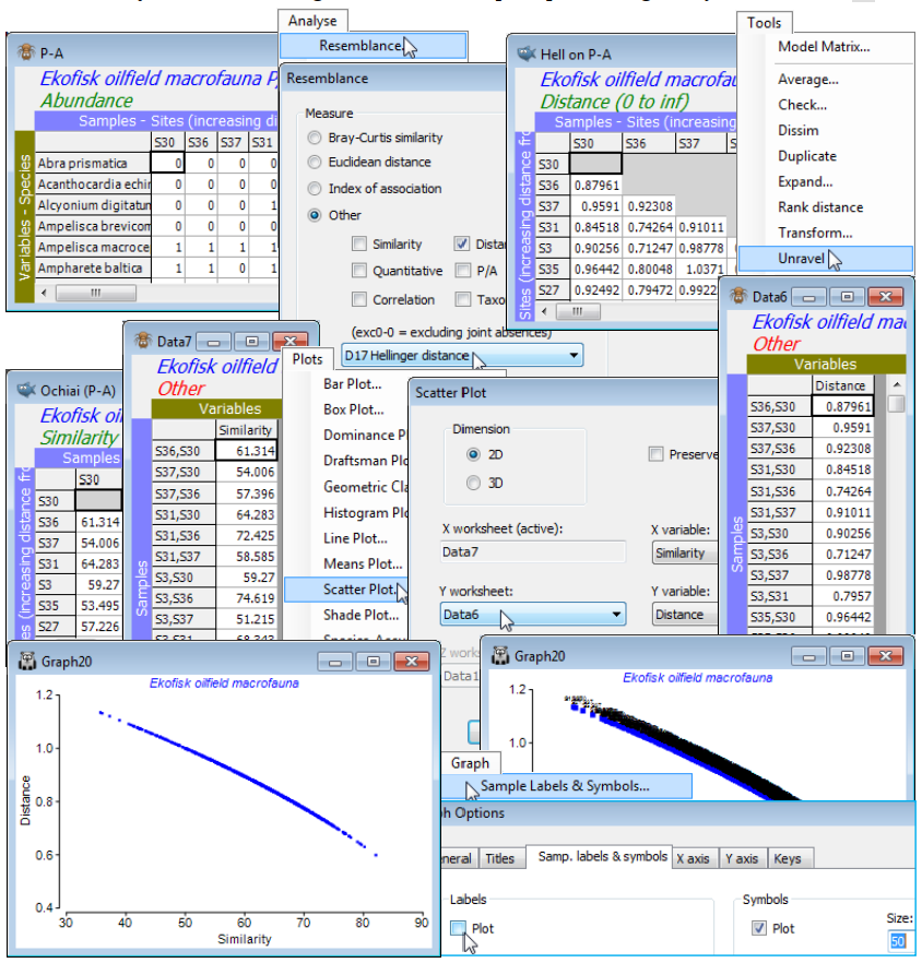
Demonstrate one of these points for the Ekofisk abundance data in the Ekofisk ws – which should still be open – by calculating Hellinger distance ($D_{17}$) on the presence/absence data produced from the macrofauna sheet, and comparing this with the Ochiai P/A coefficient ($S_{14}$). Thus:
a) With Ekofisk macrofauna counts as the active window, Pre-treatment>Transform(overall)> (Transformation: Presence/absence) to produce the P/A matrix, then renamed P-A (forward slash is not a permitted symbol in the Explorer tree, since these may sometimes be filenames);
b) On P-A, Analyse>Resemblance>(Measure•Other: D17 Hellinger distance) & (Analyse between •Samples), renaming the Resem sheet to Hell on P-A. [Do not take ‘Add dummy variable’ here – or routinely (always think carefully about it first!). It will have negligible effect here on relative distances because there are no denuded samples at all. However, the option is permitted with all measures and could make sense, in the presence of blank or near-blank samples (which are then required to have zero or near-zero distances/dissimilarities), for all those coefficients identified above (as ratios). This is essentially anything with a $y$ term or $p_{12}$ in the denominator, since these give an Undefined! resemblance entry for blank samples. The pure distance measures $D_1$, $D_6$, $D_7$ and $D_{10}$ will be unchanged with an added dummy, as will the species-standardised $S_{15}$ (which promptly has to remove the just-added dummy variable since its range $R_i$ over samples is zero!)]
c) On Ekofisk macrofauna counts take Analyse>Resemblance>(Measure•Other:S14 Ochiai(P/A)), renaming the result to Ochiai (P/A).
To view the relationship between these matrices, exploit two of the new features in PRIMER 7:
d) Run Tools>Unravel on both Hell on P-A and Ochiai (P/A), to turn these triangular matrices into long single columns (unravelling the rows), possibly now called Data6 and Data7.
e) With Data7 (say) as the active sheet, take Plots>Scatter Plot>(Dimension•2D) & (X variable: Similarity) & (Y worksheet: Data6) & (Y variable: Distance) – of course the X worksheet is the active Data7 – to see that Hellinger distance (on P/A data) is a decreasing function (near-linear here) of Ochiai similarity. The unnecessary sample labels can be removed by Graph>Sample Labels & Symbols, unchecking Labels✓Plot, and perhaps reducing the Symbols to Size: 50.
Other coefficients
Returning to the quantitative resemblance coefficients in the •Others list, five further measures given under the ✓Distance/dissimilarity heading are (loosely) based on likelihood-ratio tests. All are motivated by the (usually unrealistic) model in which the individuals of a species are randomly distributed in space or time (i.e. the data are strict counts, Poisson distributed), independently of other species, and with the mean count differing over species. A generalised likelihood ratio (GLR) test that two samples come from the same assemblage then produces the test statistic:
$D^{BinD} = 2\sum_i \left[ y_{i1} \log \left( \frac{y_{i1}}{ y_{i1}+y_{i2}} \right) + y_{i2} \log \left( \frac{y_{i2}}{ y_{i1}+y_{i2}} \right) + \left( y_{i1} + y_{i2}\right) \log 2 \right] \text{\hspace{10mm} Binomial deviance,} $
where the sum is over all $p$ species as usual (note the first two terms do go to zero, unambiguously, when $y_{i1}$ and $y_{i2}$ are zero, respectively). In fact, the coefficient is of the form $2 \sum \left[ O \log(O/E) \right]$, where $O=y_{i1}$ or $y_{i2}$ and $E=(y_{i1}+y_{i2})/2$ are the observed and expected values in a chi-squared type test of equality of counts for species $i$, then summed over the (supposedly independent) species, $i = 1,\ldots, p$. The more familiar Wald test statistic for this situation is $\sum \left[(O – E)^2 /E \right]$, but the two measures are likely to behave very similarly in practice (both having large-sample distributions of $\chi^2$ on $p$ df). A more useful variant of the latter is therefore given under Measure•Others, by simply dividing the chi-squared by the number of non jointly-absent species ($p_{12}$) for these two samples:
$D^{Wald} = \frac{1}{p_{12}} \sum_i \left[ \frac{ \left( y_{i1}-y_{i2} \right)^2}{ \left( y_{i1}+y_{i2} \right)} \right] \text{\hspace{30mm} Wald (chi-squared) coefficient,}$
thus making this form of the coefficient independent of joint absences. This could be further modified in a natural way, to make it more robust to large $y_{ij}$ (outliers) whilst preserving similar behaviour, by replacing a sum of squares with a sum of absolute values:
$D^{Chi} = \frac{1}{p_{12}} \sum_i \left[ \frac{ \left| y_{i1}-y_{i2} \right|}{ \sqrt {y_{i1}+y_{i2}}} \right] \text{\hspace{30mm} ‘Chi’ statistic.}$
All three coefficients above are not dimensionless, i.e. they make sense only when applied to real counts and not densities, biomass, area cover etc. Millar RB & Anderson MJ 2004, J Exp Mar Biol Ecol 305: 191-221 therefore suggest a scale-invariant form of the first one:
$ D^{SBinD} = \sum_i \frac{1}{ \left( y_{i1}+y_{i2} \right)} \left[ y_{i1} \log \left( \frac{y_{i1}}{ y_{i1}+y_{i2}} \right) + y_{i2} \log \left( \frac{y_{i2}}{ y_{i1}+y_{i2}} \right) + \left( y_{i1} + y_{i2}\right) \log 2 \right] $ $\text{\hspace{95mm} Binomial deviance (scaled).} $
(They choose to drop the 2 outside the sum and work in logs to the base 10, so for consistency with that paper, PRIMER does the same. Resulting analyses would be unchanged either way, since the difference is just the same constant multiplier for all pairs of samples). Because of the close link between likelihood ratio and Wald statistics, $D^{SBinD}$ is seen to be a form of Clark’s divergence, $D_{11}$, though without the adjustment for double zeros that comes through the $p_{12}$ divisor.
Cao Y, Bark AW, Williams WP 1997, Hydrobiologia 347: 25-40 suggested a coefficient which has been advocated or used in subsequent studies. It looks very reminiscent of the (scaled) likelihood ratio statistic, but with an important switch of the $y_{i1}$ and $y_{i2}$ inside the logs:
$ D^{CY} = -\frac{1}{p_{12}} \sum_i \frac{1}{ \left( y_{i1}+y_{i2} \right)} \left[ y_{i1} \log \left( \frac{y_{i2}}{ y_{i1}+y_{i2}} \right) + y_{i2} \log \left( \frac{y_{i1}}{ y_{i1}+y_{i2}} \right) + \left( y_{i1} + y_{i2}\right) \log 2 \right] \text{\hspace{5mm} CY.} $
(It does take positive values in spite of the negative sign outside the sum!). Like $D^{Wald}$ and $D^{Chi}$, it too contains the important $p_{12}$ denominator adjustment to ignore joint absences, which the binomial deviance measures omit, but like $D^{SBinD}$ it adds a denominator scaling to make the measure scale-invariant. However, it is now undefined when either $y_{i1} = 0$ (and $y_{i2} \ne 0$) or vice-versa, which could be much of the time, in fact! Zeros have to be replaced with a small positive number therefore, and the outcome is sensitive to this choice. No theoretical basis has been advanced for this coefficient, and it does not have an intuitively simple form, so any good operational properties it may possess must be somewhat fortuitous, and it is probably best avoided by the novice user.
Between-curve distances
Another useful application of multivariate methods was touched on at the end of Section 4, namely the analysis of structured sets of curves or (pseudo-)frequency distributions, generically referred to as sample profiles. These include particle- or body-size analyses, or growth curves, with several replicate profiles from each of a number of sites, times, treatments etc. Simple univariate statistical treatment of the size variable is often impossible because of the inherent serial correlation problems (repeated measures) of, for example, tracking the body size of a single organism through time, or the lack of a proper frequency distribution structure in histograms of particle sizes (in no sense are we counting independent particles entering the sampling device, to give multinomial frequencies). A viable multivariate alternative is to treat the independent units as the whole profiles and define distances among them, taking these pairwise resemblances into, say, the ANOSIM tests discussed in Section 9. Suitable distance measures between pairs of curves include Euclidean distance $D_1$ (or its square), the Manhattan distance $D_7$ and, specifically for comparing cumulative curves:
$D^{\max} = \max_i | y_{i1} - y_{i2} | \text{ \hspace{35mm} Maximum distance,} $
which is also a Distance/dissimilarity option on the •Others list. The maximum departure of two cumulative frequency curves from each other, taken over all the size categories, is the basis of the Kolmogorov-Smirnov test, but the testing structure there relies on real (multinomial) frequencies. Where this is not the case, as often, maximum departure may still be a sensible distance measure of two curves to feed into multivariate analysis, though Manhattan (or Euclidean) distance is likely to be at least as good, since it sums positive contributions across the entire size range.
(Plymouth particle-size analysis)
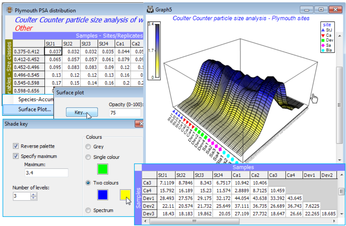
An example of a particle-size analysis (PSA) matrix has already been seen for Danish sediments at the end of Section 4, for which the histogram was smoothed by cumulating the size-classes. Here we examine instead an already smooth frequency distribution from Coulter Counter processing of water samples, in which large numbers of suspended particulates are automatically sized into one of 92 logarithmically increasing particle-diameter ranges (the variables). The samples are of four replicate water samples from each of five Plymouth sites, and some analysis is presented towards the end of Chapter 8 of CiMC. The directory C:\Examples v7\Plymouth PSA holds the frequency distributions in Plymouth PSA distribution. Columns are samples, and entries are % particles in each size-class (add to 100). The curves are conveniently viewed with Plots>Surface Plot, colour changed with Graph>Special>Key, zoomed with Graph>Zoom In or the  icon, and rotated with Graph>Rotate Axes or the
  icon (hold-click and move cursor). Create Manhattan distances among the curves, with Analyse> Resemblance>(Measure•Other: D7 Manhattan distance), which could go into ANOSIM to test for characteristic site differences in PSA profiles at these times.
Taxonomic distinctness/ aggregation files
A later section (15) discusses univariate diversity indices that can be computed from each sample, including biodiversity measures that are based on the relatedness of the species making up a simple species list (P/A data), see Chapter 17 of CiMC. Though the supplied relatedness could be genetic, phylogenetic or functional – through suitable provision of a distance/dissimilarity matrix among the species, perhaps (but not necessarily) their pairwise distances apart through some hierarchical arrangement of species – PRIMER 7 implements the idea mainly in terms of taxonomic distinctness (see Section 15). These are the distances travelled in connecting every pair of species through a tree with a fixed set of levels (typically, a Linnaean taxonomy). If, on average, these distances are large, then the sample is considered biodiverse. A necessary input is a variable information sheet, which (for historic reasons) PRIMER calls an aggregation file (see the end of Section 2), defining the taxonomy – which species belong to which genera, families, orders, etc. From this, path weights $\omega_{ij}$ are calculated between every pair of species, $i$ and $j$. Always, $\omega_{ij}$ takes the value 100 for two species that are connected at the most distant level; e.g. if the final column heading in the taxonomy file is phylum then two species in different phyla are defined to be 100 units apart (do not add a final column, say kingdom, for which all species have the same entry, Animalia; you could then only attain the value 100 for species in different kingdoms). By default, intervening levels are considered to be equally-spaced. For example, for a hierarchy of species from different classes all in the same phylum, with the five levels of species, genus, family, order and class, two species in the same genera are 20 units apart, in different genera but the same family are 40 units apart, etc. This can be overruled in two ways: either a user can define his/her own step branch-lengths, which will again be rescaled to a maximum of 100 for two species in different top-level groups, whatever scale is input for the absolute steps; or the information in the aggregation matrix about taxon richness at each hierarchical level can be used (a level in the tree which has almost as many taxa as the level below it gives rise to a step of shorter branch-length).
Taxonomic dissimilarity measures
This concept of taxonomic distinctness can be carried over from a diversity index to a dissimilarity coefficient. Two measures are given under Analyse>Resemblance>(Measure•Other: ✓Taxonomic P/A). Both are presence/absence measures only, indicated by the plus sign superscript: $\Gamma^+$ (upper case Greek gamma) is a natural extension of Bray-Curtis dissimilarity on P/A data (the latter is just the complement of Sørensen $S_8$), and $\Theta^+$ (upper case Greek theta) similarly extends Kulczynski P/A dissimilarity, the complement of $S_{13}$. They are formally defined as:
$\Gamma^+ = \frac{ \left( \sum_{i=1}^{s_1} \min_j \left\{ \omega_{ij} \right\} + \sum_{j=1}^{s_2} \min_i \left\{ \omega_{ij} \right\} \right) }{ \left( s_1 +s_2 \right) } \text{, \hspace{8mm}} \Theta^+ = \frac{1}{2} \left( \frac{ \sum_{i=1}^{s_1} \min_j \left\{ \omega_{ij} \right\} }{ s_1} + \frac{ \sum_{j=1}^{s_2} \min_i \left\{ \omega_{ij} \right\} }{ s_2} \right) $
where there are $s_1$ species present in sample 1 and $s_2$ in sample 2, and $\omega_{ij}$ is the distance through the tree from species $i$ of sample 1 ($i =$ 1, 2, …, $s_1$) to species $j$ of sample 2 ($j =$ 1, 2, …, $s_2$). This is almost simpler to express in words: for each species one finds the most closely related species in the opposite sample, then averages these minimum path lengths over all ($s_1 + s_2$) species, to obtain $\Gamma^+$. (If the nearest relation in the opposite sample is the same species, the path length is defined to be zero, of course). For $\Theta^+$, these averages are calculated separately, i.e. the average path length for all species in sample 1 to their nearest neighbours in sample 2, then for all species in sample 2 to their nearest neighbour in sample 1, with these two averages then themselves being averaged.
As noted, these constructions result in $\Gamma^+$ and $\Theta^+$ reducing to the dissimilarity forms of Sørensen and Kulczynski (P/A) when the hierarchy collapses, i.e. when all species are in one higher-order group and the path lengths are 0 or 100 (species do or do not have a match in the opposite sample).
$\Theta^+$ was defined (and referred to as an ‘optimal mapping statistic’, denoted $M$) by Clarke KR & Warwick RM 1998, Oecologia 113: 278-289, and $\Gamma^+$ is (to within a constant) the TD of Izsak C & Price ARG 2001, Mar Ecol Prog Ser 215: 69-77. They are clearly closely related, and will be identical when $s_1=s_2$. Their use is in ordinating samples from widely-spread biogeographic regions with few, if any, shared species, but which will always have higher-order taxa in common. They also provide a certain amount of robustness in dissimilarity value to mistakes or inconsistent identification at the finest taxonomic levels (see CiMC, end of Chapter 17, for two applications from Clarke KR, Somerfield PJ, Chapman MG 2006, J Exp Mar Biol Ecol 330: 55-80).
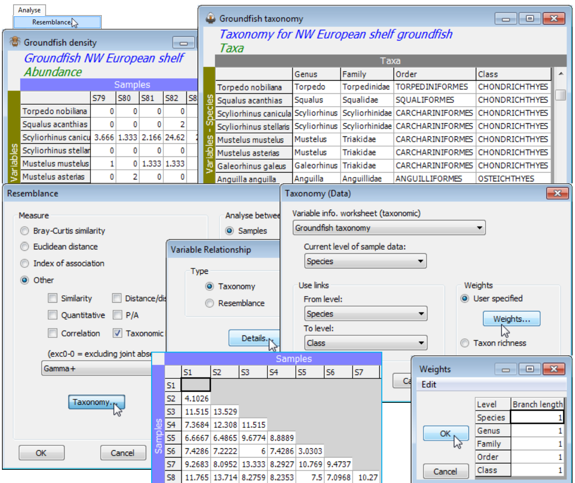
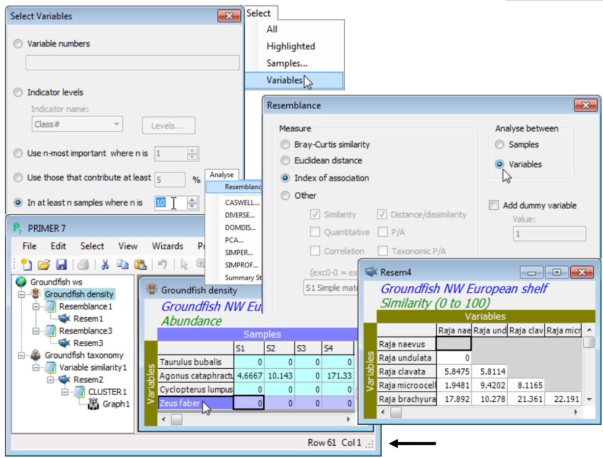
(Groundfish of European shelf waters)
Assemblage data from 93 groundfish species, those that could be reliably sampled and identified in beam-trawl surveys by research vessels from several countries surrounding NW European shelf waters, were analysed by Rogers SI, Clarke KR, Reynolds JD 1999, J Anim Ecol 68: 769-782. The data matrix, C:\Examples v7\Europe groundfish\Groundfish density(.pri) is of 277 locations (ICES quarter-rectangles) sampled in the third quarter of the year over the period 1990-96, with the values being mean catch rates corrected to number of fish per 8m beam trawl per hour. The sites are divided a priori into 9 coastal areas (1 to 9 in factor area: 1=Bristol Channel, 2=Western Irish Sea, ..., 9=E Central North Sea, see the Edit>Properties box). Also available is a PRIMER format variable information file, the aggregation sheet, Groundfish taxonomy(.agg), met briefly at the end of Section 2. Open both into a new workspace and on Groundfish density Analyse>Resemblance> (Analyse between•Samples)&(Measure•Other: Gamma+>Taxonomy>(Type•Taxonomy)>Details >(Variable info. worksheet (taxonomic): Groundfish taxonomy)), accepting all defaults on this last dialog box – though you might like to take User specified>Weights to note how the step lengths between levels are set to be equal, resulting in path lengths between species of 0, 20, 40, 60, 80, 100, as earlier described. Alternatives might be to flatten the tree at the top, by setting the final step (Class) to 0, or to give more weight to the fine-level taxonomy, with decreasing entries 5, 4, 3, 2, 1.
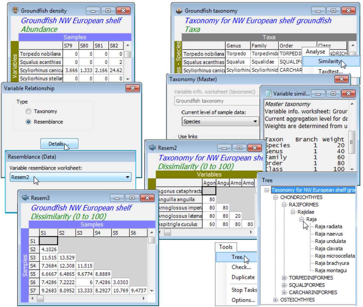
Relatedness supplied as resemblances
Note the alternative means of supplying the variable information, to these dissimilarity measures and the biodiversity indices of Section 15, which is now available in PRIMER 7. In the Variable Relationship dialog box, Type•Resemblance>Details now requires specification of a numeric among-species resemblance matrix which could be constructed from genetic, functional, etc. data, but is illustrated here by first creating a species distance matrix through the Linnean tree with Analyse>Similarity when the aggregation file Groundfish taxonomy is the active window. This takes you to a similar Taxonomy dialog box as above and creates sheet Resem2 of among-species distances 20, 40, 60, 80, 100. The Linnean tree could be viewed by Analyse>Cluster (next section) on Resem2, or in alternative format by Tools>Tree on Groundfish taxonomy. When Resem2 is supplied as the Variable resemblance worksheet from Details, the same $\Gamma^+$ matrix results, naturally.
Analysing between variables
The introduction above of the concept of ‘distances’ among species raises the issue of how best to compute species similarities – or more generally variable associations – taking the menu option of Analyse>Resemblance>(Analyse between•Variables). Several significant new developments in PRIMER 7 (see Section 10 and Chapter 7 of CiMC) on shade plots and coherent species curves concern better display and analysis techniques for characterising responses of individual (or groups of) species across the samples in space, time or over a changing environment. Two species are considered perfectly similar if they co-occur across samples – with numbers or biomass in strict proportion, for quantitative data. As with sample similarities, the issue of how to treat joint absence is often relevant here too – it would often be appropriate to regard the absence of two species at a particular site as uninformative (a clay-living and a gravel-living species are not similar because neither are found at sandy sites). A measure which captures this biological constraint well is the Whittaker Index of Association (IA), met earlier in this section. As remarked then, this will give the same outcome as standardising species (by total) and applying Bray-Curtis on the species. The (implicit) standardisation however will come unstuck with all-blank species, which must certainly be removed, and it is also almost always a good idea to remove all the ‘occasional’ species, rarely observed and with low abundances when they do occur. The various options for reducing to the ‘most important’ species were covered at the end of Section 3, and for standardising species near the start of Section 4; these options would not usually apply when calculating sample similarities, but are important to eliminate wildly erratic, and not meaningful, similarities among rare species.
On the Groundfish density matrix, Select>Variables>(•In at least n samples where n is: 10). To see how many species are retained (61, in fact), click on the sheet’s final row which displays this in the status bar at the foot of the PRIMER desktop. Take Analyse>Resemblance>(Measure•Index of association) & (Analyse between•Variables) to create the species similarities (Resem4 perhaps). Show that the same outcome is produced (Resem5) by putting the selected species from Groundfish density through Pre-treatment>Standardise>(Standardise•Variables) & (By•Total), followed by Analyse>Resemblance>(Measure•Bray-Curtis similarity) & (Analyse between•Variables).
Correlation between variables
One context in which resemblances between variables is often of primary interest is in dealing with environmental variables, biomarkers, morphology etc. Concepts of ignoring joint absences do not apply – in fact zero no longer necessarily means absence (e.g. $0^\circ$C), particularly after normalisation (see Section 4). Variables are usually on different measurement scales (or are non-comparable on the same units), so correlation is a natural choice, with its built-in normalisation. The final option in Measure•Others is ✓Correlation, with seven variations of a correlation coefficient, $\rho$, namely
$\rho ^P = \frac{ \sum_j \left( y_{1j}-y_{1\bullet} \right)\left( y_{2j}-y_{2\bullet} \right) }{ \sqrt{ \sum_j \left( y_{1j}-y_{1\bullet} \right)^2 \sum_j \left( y_{2j}-y_{2\bullet} \right)^2}} \text{ \hspace{14mm} Pearson (product-moment) correlation,} $
where $y_{1\bullet} = \left( \sum_j y_{1j} \right)/n$ is the average of the $n$ sample readings for variable 1, etc., and two non-parametric choices, based only on rank values ($r_{ij}$), the numbers 1, 2, 3, .., n across samples $j$, for each variable $i$. Spearman is simply Pearson correlation calculated on the ranks, reducing to:
$\rho^S = 1 - \frac{6}{n \left(n^2-1 \right) } \sum_j \left( r_{1j} - r_{2j} \right)^2 \text{ \hspace{10mm} Spearman rank correlation,} $
and Kendall’s $\tau$ is an alternative (Kendall MG 1970, Rank correlation methods, Griffin, London), which in practice tracks Spearman closely, but with lower absolute values. These three coefficients are then given as absolute values, $| \rho |$, to cater for situations where it is not especially meaningful to distinguish between positive and negative correlations (e.g. some biomarkers increase under impact and some decrease, so an absolute $\rho$ is often a better description of their inter-relationship). A final weighted form of Spearman gives more emphasis to small ranks (high variable values):
$\rho^W = 1 - \frac{6}{n \left(n-1 \right) } \sum_j \frac{ \left( r_{1j} - r_{2j} \right)^2 }{ r_{1j} + r_{2j} } \text{ \hspace{16mm} Weighted Spearman rank correlation,} $
but this really only makes sense in an asymmetric context, such as correlating the entries of two resemblance matrices, thus emphasising matching pairs of high similarities – see the discussion of equation (11.4) in CiMC.
Correlation as similarity
Use of a correlation matrix between all pairs of variables as input to a multivariate ordination (say), in which points denote variables rather than samples (so that highly correlated variables are placed close together), either requires one of the absolute coefficients or a simple shift $S = 50(1+\rho)$ of the three standard coefficients, so that they are defined over (0, 100) rather than (–1, 1). There is an important difference between the two approaches: should highly negatively correlated variables be considered highly similar (use an absolute measure) or highly dissimilar (shift the scale upwards)? The practical context should usually make clear which is the right choice.
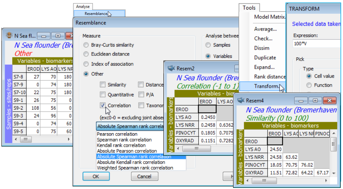
Save and close the current Europe groundfish workspace (as Groundfish ws), and open that for the N Sea biomarkers N Sea ws, created towards the end of Section 4 – see there for description of the variables. (If not available, just open N Sea flounder biomarkers(.pri) from directory C:\Examples v7\N Sea biomarkers). The previous pre-treatment by variability weighting of these (transformed) biomarkers was designed for calculation of standard sample similarities (which you may now wish to do by Analyse>Resemblance>(Measure•Euclidean distance) & (Analyse between•Samples)), but the reason for re-opening this workspace now is to calculate similarities among variables, via correlation. The choice is between standard (Pearson) correlation and a rank-based correlation (Spearman, say); if the analysis includes the categorical as well as the continuous variables, the rank option may be preferred. Note that any variability weighting previously carried out, to weight the biomarkers against each other in calculating sample similarities, will be irrelevant to correlation computation of variable similarities, because variables are renormalised (under Pearson) or ranked (under Spearman). For Spearman, even the square root transform applied to the EROD and Lipid variables is irrelevant, since this will not change the rank order of variable values across samples. Note that low lysosomal stability (AO or NRR) is associated with high EROD etc. – both indicating contaminant impact – so an absolute correlation measure is used to capture biomarker similarities. Analyse>Resemblance>(Measure•Other>✓Correlation: Absolute Spearman rank correlation) & (Analyse between•Variables) on N Sea flounder biomarkers will produce values in the range (0,1). These could be scaled to (0,100) using Tools>Transform>(Expression:100*V) – see box heading Transform on resemblances in Section 11 – and the Type changed from Correlation to Similarity with Edit>Properties>(Resemblance type•Similarity) but this is not practically necessary for most routines in PRIMER, such as nMDS ordination, since only ranks of the resemblances are used.
Corrections for missing data
Returning to the main purpose of resemblance measures, to describe similarity among samples, an important new feature in PRIMER 7, not offered in earlier versions, is that resemblance measures will now be calculated in the presence of missing cells (identified by Missing! in the sheet). As described in Section 1 (box heading Missing or zero values?) this tends to arise only for sheets of type Environmental or Other – species matrices can have whole samples missing from an otherwise balanced layout but this is not regarded as missing data, just unbalanced design, handled routinely in PRIMER (and PERMANOVA+). Under restrictive conditions (multivariate normality in a ‘not too high’ dimensional space) it may be possible for some environmental data to estimate single entries missing at random, utilising the correlations between variables (see Tools>Missing in Section 12) but in many contexts for which missing entries are almost guaranteed, these modelling conditions will not apply. An example would be would be questionnaire data, in which the samples are the individual respondents and the variables the questions, e.g. with matrix entries 1 to 5, for a ‘disagree strongly’ to ‘agree strongly’ scale. This is a likely area for application of multivariate methods, calculating similarities between respondents in the profile of answers, and linking this to demographic/socio-economic data, e.g. PRIMER applications from environmental economics exist, but missing answers are commonplace and probably not estimable under normality assumptions.
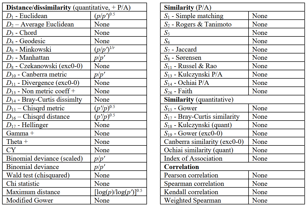
Where there is missing data, PRIMER 7 therefore computes a resemblance between each specific pair of samples by removing (for that calculation only) those variables in which one or other value is missing (referred to as pairwise elimination of missing data). This can cause a crude bias in some distance measures which are in the form of sums rather than averages of variable contributions, in that pairs of samples with many missing entries will automatically return lower distances than those with few or no missing values, all else being equal. Examples are Euclidean ($D_1$) or Manhattan ($D_7$) distances, which are both based on simple sums over the variables. A correction for these biases is straightforward in this case: average Euclidean distance ($D_2$) clearly has no such crude bias since the contributions from each variable are averaged not summed. The solution for $D_1$ is therefore to multiply up the summation by a factor ($p/p^′$), where $p$ is the full number of variables in the array, and $p^′$ is the number of variables used in that specific sum, having pairwise-eliminated the missing variables. The outer square root in the definition of $D_1$ makes the overall correction term $(p/p^′)^{0.5}$.
PRIMER 7 automatically applies such correction factors to every resemblance measure, if needed, as shown in the following table. Note that the standardisation implicit in many measures, including all (dis)similarities, avoids the need for correction, sample totals always being re-defined for each pairwise-eliminated set. The corrections have only asymptotic justification for the more complex measures, e.g. $D_{16}$ Chisquared distance for which the correction term is $(p^′/p)^{0.5}$, not $(p/p^′)^{0.5}$, thus a downward adjustment. (Similarly, that for Maximum Distance is based on Jensen inequalities on asymptotics of extreme value distributions so is definitely approximate!). It should be stressed that these corrections assume an average contribution from each missing variable, as measured by the average for the present variables. Broadly, this is not unreasonable if values are missing at random, but is theoretically inferior to reconstruction of missing values by Tools>Missing, when the strict conditions for this apply, since that uses variable correlations to estimate non-average values.
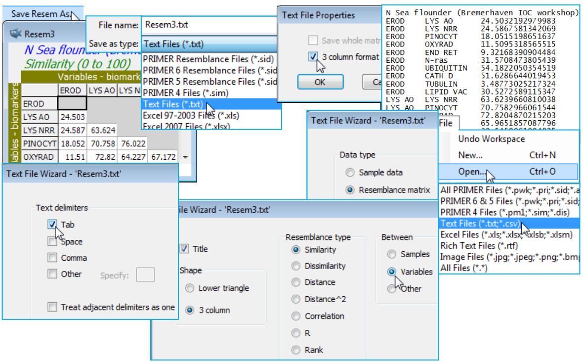
Saving & opening triangular matrices
File>Save Resem As will save a resemblance matrix in internal binary PRIMER v7 (*.sid) format, though the previous v6 and v5 binary formats (also *.sid) are other options – as is the early DOS text format (*.sim) – all likely to be of limited utility now. More useful are the options to save the triangular matrix as an Excel sheet (*.xls or *.xlsx), in which case the diagonal and upper triangular cells are left blank. Several text file choices (*.txt) are also offered: by default a lower triangular matrix is output with tabs as separators, though there is also the option to output a ‘whole matrix’, i.e. a full square is saved, with filled diagonals and upper triangle as the transpose of the lower half. Another interesting possibility is a 3-column output format, with first and second columns giving the row and column labels for the lower triangle, and the third column the resemblance entry. (This parallels the 3-column – flat-form or record format – data files, the output or input of which was seen in Section 1). These options should, between them, make it easy to take a resemblance matrix out of PRIMER into other software, if needed.
File>Open>(Data type•Resemblance matrix) gives all these options in reverse (and more), for reading in any triangular matrix. Generic questions concern the existence or otherwise of a ✓Title, and a type specification of: •Similarity/ •Dissimilarity /•Distance /•Distance$^2$ /•Correlation /•R /•Rank (the notation R come from pairwise ANOSIM statistics, see Section 9, but could represent any measure defined over (-1, 1) for which the larger the value the greater the ‘distance apart’). Whether input matrices are to be treated as (Between•Samples) or (Between•Variables) is also required, of course. Excel files (*.xls or *. xlsx) are assumed to be in lower triangular form – if an upper triangle or diagonal is present it is ignored. Text files have more options, the choices being: (Shape•Lower triangle) or (Shape•3 column). Both of these lead to the same ‘Text File Wizard’ dialog seen in Section 1 for inputting data matrices, in which any form of separator between entries can be defined, even in combination. [Thus, though of limited usefulness, if unravelled distance matrices – as created for the scatter plot of (Hellinger on P/A) vs. (Ochiai P/A) earlier in this section – were saved as *.txt data files (of two columns), with care they could be read back into PRIMER to reform the triangular matrices. To do this, you would need to say you are inputting resemblances in 3-column format, and take both ✓Tab and ✓Comma as Text delimiters, allowing interpretation of the 1st column (‘row label,col label’) as columns 1 and 2 of the 3-column format.]
Try saving the previously created ‘variable similarities’ matrix among biomarkers (from the N Sea ws workspace which should still be open) into Excel and text formats, in both standard *.txt and the 3-column *.txt formats. Look at these in Word or Notepad, and then try re-opening them again in PRIMER. Resave the workspace, N Sea ws, for a later section and close it.