7. Managing the workspace and plotting (Window, File, View, Multi Plot, Plots)
- Explorer tree
- Forward and backward propagation
- Closing, redisplaying & tiling windows; Minimising windows; View menu
- Understanding the Explorer tree
- Rolling up branches of the tree
- Renaming or deleting items in a workspace; Undo in the Explorer tree to reinstate or re-order
- Saving plots
- Vector vs. pixel plots
- Saving graph values; Saving results
- Adding notes
- Printing results and graphs
- Automatic creation of multi-plots
- User creation/ manipulation of multi-plots
- Plots menu
- Workspace planning
Explorer tree
It will have been obvious from performing the worked examples of the previous sections that the structure of all calculations in the current workspace is stored and displayed in logical fashion, on the left of the PRIMER desktop, in the Explorer tree. This lists data sheet names, and any derived constructions (such as further data sheets ![]() , resemblance matrices
, resemblance matrices ![]() or plot windows
or plot windows ![]() ), via the intermediate Results windows
), via the intermediate Results windows  , which are simple text windows giving details of the options taken in moving down a branch from one sheet to an ensuing window, in addition to listing textual results of the operation. This allows the user to manage the workspace, finding and activating only windows which are needed, and saving the entire workspace structure in a single operation, and in a single file
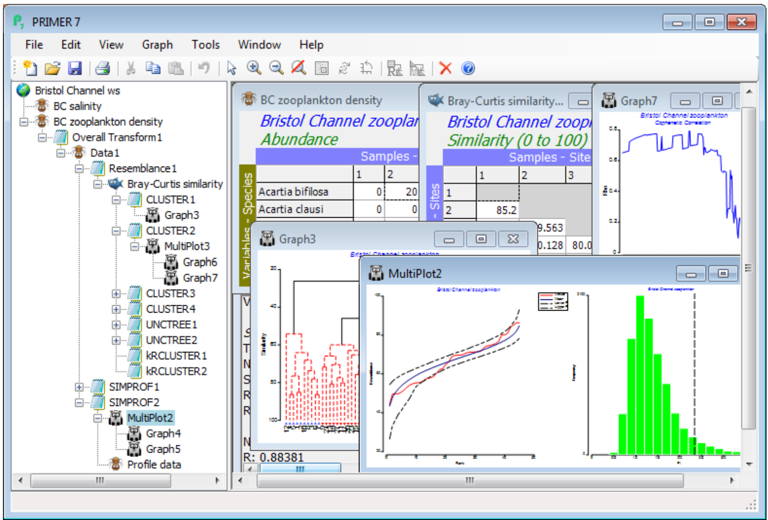
 ![]() , for later retrieval. For example, if you have been analysing the data of the previous section, the PRIMER desktop should now look something like:
, for later retrieval. For example, if you have been analysing the data of the previous section, the PRIMER desktop should now look something like:
Forward and backward propagation
The Explorer tree not only makes it easy to navigate the sequence of steps taken in an analysis but also, importantly, reflects the program’s internal knowledge of the inter-relationships among data, resemblance sheets and plot windows. It uses this structure to select sensible defaults, and even occasionally to reach back and find a data matrix higher up the same branch, needed for a specific operation. (An example of this has been seen in running SIMPROF from the various clustering methods – these routines are all launched with a resemblance matrix as the active sheet, but the tests require permutation of rows or columns of the preceding data matrix).The Explorer tree is also used for forward and backward propagation of factor/indicator information, along a single branch of the tree. A factor’s properties, such as symbol types for each level, are naturally passed down a branch as new data sheets or plots are formed from the data sheet for which that factor was created. The reverse is also true: definition of new factors, produced from an editing step on a plot, will typically be passed back to the data matrix at the head of that branch, and then down other branches leading from the original sheet. But such information is not passed from one branch to a distinct branch (factors can be retrieved from distinct branches by Edit>Factors>Import), and there are also natural blocks to propagation. For example, if a Tools>Average (or Sum or Merge) operation – see Section 11 – is carried out part way down a branch, PRIMER 7 (unlike PRIMER 6) will now place the resulting averaged sheet on the same branch as its parent matrix, and all factors will be passed forward to the condensed sheet (though some factors may have undefined entries if the averaging has been over levels which differ for those factors). However, changes now to factors of the condensed matrix clearly cannot sensibly be backward propagated to the original larger sheet.
Closing, redisplaying & tiling windows; Minimising windows; View menu
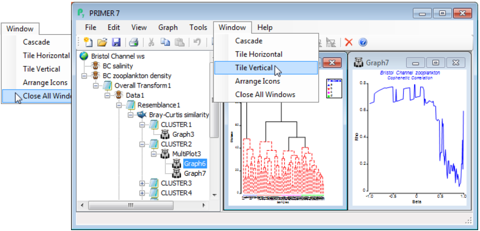
From the Explorer tree for the above illustration, you can see that workspace has been saved as Bristol Channel ws, with every row below this representing a window in the workspace, whether open or not. It is important to appreciate that whilst you can close down windows – individually by the usual  icon (top right), or all of them at once with Window>Close All Windows – they will remain in the workspace, and can simply be re-displayed by clicking on their name (or icon) in the Explorer tree. The option to tile or cascade windows may also be useful here, so that a common way of tidying up the display area (right panel of the PRIMER desktop) is to close all windows, click on the Explorer tree names for the ones you want to re-display and then take Window>Tile Horizontal or Tile Vertical or Cascade.
For consistency with much earlier PRIMER versions and other Windows software, there is also an option to minimise a window to the bottom of the PRIMER desktop, by clicking on the minimising icon  , but this is no longer necessary or useful with more recent versions of PRIMER, it being easier simply to close the window and retrieve it from the Explorer tree when required.
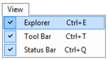
There will be situations in which, in order to display as much of a plot or datasheet on screen as possible, it is desirable to temporarily hide some of the other features, to widen and heighten the display area. In standard Windows fashion, the View menu allows three features to be toggled off and on again: ✓Explorer (the left panel), ✓Tool Bar (icons in the top row) and ✓Status Bar (bottom row, used to display position of the cursor in a data matrix, progress of a calculation etc.).
Understanding the Explorer tree
Understanding the Explorer tree, however, is the key to managing your work pattern in PRIMER. In the above workspace, click on the successive entries. After the workspace name (![]() Bristol Channel ws) two data matrices have clearly been opened into the workspace,
Bristol Channel ws) two data matrices have clearly been opened into the workspace, ![]() BC salinity (a repeat of the salinity information for each site but in the form of a separate environmental matrix, rather than a factor of the zooplankton array – this will be useful later when displaying bubble plots of salinity on an MDS plot), and the community data
BC salinity (a repeat of the salinity information for each site but in the form of a separate environmental matrix, rather than a factor of the zooplankton array – this will be useful later when displaying bubble plots of salinity on an MDS plot), and the community data ![]() BC zooplankton density. A fourth-root transform has been taken, indicated in the Overall Transform1 results window, giving
BC zooplankton density. A fourth-root transform has been taken, indicated in the Overall Transform1 results window, giving ![]() Data1. The similarity calculation follows: Resemblance1 shows that this was Bray-Curtis, calculated for all samples using all species, to give the triangular resemblance sheet – by default this would be Resem1 but has been renamed (e.g. by clicking twice on the name) to
Data1. The similarity calculation follows: Resemblance1 shows that this was Bray-Curtis, calculated for all samples using all species, to give the triangular resemblance sheet – by default this would be Resem1 but has been renamed (e.g. by clicking twice on the name) to ![]() Bray-Curtis similarity on 4th root. Renaming important windows in this way is always a useful aid to navigating around a large workspace (and more of this should probably have been carried out in the current example!). The agglomerative (Group Average) cluster analysis generates the CLUSTER1 results window and the dendrogram plot,
Bray-Curtis similarity on 4th root. Renaming important windows in this way is always a useful aid to navigating around a large workspace (and more of this should probably have been carried out in the current example!). The agglomerative (Group Average) cluster analysis generates the CLUSTER1 results window and the dendrogram plot, ![]() Graph3, the number indicating that two other graphs were produced before this (in an analysis from Section 6, under SIMPROF1 lower down the Explorer tree, on a branch stemming back to the transformed Data1 sheet rather than from the Bray-Curtis similarity matrix). Note that all these steps, which create a derived sheet or plot file, possess an intervening results window. This is what distinguishes operations on the Pre-treatment, Analyse, Plots and Tools menus (and PERMANOVA+, if installed) from those under File, Edit or Select. The latter do not produce new, derived sheets or intervening results windows, but make changes (temporary or permanent) to the currently active sheet.
Graph3, the number indicating that two other graphs were produced before this (in an analysis from Section 6, under SIMPROF1 lower down the Explorer tree, on a branch stemming back to the transformed Data1 sheet rather than from the Bray-Curtis similarity matrix). Note that all these steps, which create a derived sheet or plot file, possess an intervening results window. This is what distinguishes operations on the Pre-treatment, Analyse, Plots and Tools menus (and PERMANOVA+, if installed) from those under File, Edit or Select. The latter do not produce new, derived sheets or intervening results windows, but make changes (temporary or permanent) to the currently active sheet.
Rolling up branches of the tree
In the display of the Explorer tree at the beginning of this section, the SIMPROF1 window was prefaced by the rolled-up icon ![]() , and it is necessary to click on this to expand the branch below this point, replacing the rolled-up icon with one indicating that the branch is now rolled-out
, and it is necessary to click on this to expand the branch below this point, replacing the rolled-up icon with one indicating that the branch is now rolled-out ![]() (in this case to reveal a multi-plot and the two plots, Graph1 and Graph2, which have been collected together under this multiple plot construction, new to PRIMER 7, see below). A second click will reverse this operation, rolling up the branch below that point. This may be a useful way of keeping secondary analysis strands available in the workspace, but without allowing their detailed steps to clutter up the main sequence of analyses displayed in the Explorer tree. Any windows which have been closed in the PRIMER desktop (not deleted from the workspace), e.g. by an individual or a full Window>Close All Windows operation, at the time the workspace is saved, will appear only under a rolled-up entry when the workspace is re-opened. As we saw earlier (in Section 1, under the Saving, closing & opening a workspace heading) there is a new option to open a workspace with all its branches in rolled-up form, irrespective of how the workspace was saved – thus opening the workspace more quickly – requiring a succession of roll-outs to display individual sheets.
(in this case to reveal a multi-plot and the two plots, Graph1 and Graph2, which have been collected together under this multiple plot construction, new to PRIMER 7, see below). A second click will reverse this operation, rolling up the branch below that point. This may be a useful way of keeping secondary analysis strands available in the workspace, but without allowing their detailed steps to clutter up the main sequence of analyses displayed in the Explorer tree. Any windows which have been closed in the PRIMER desktop (not deleted from the workspace), e.g. by an individual or a full Window>Close All Windows operation, at the time the workspace is saved, will appear only under a rolled-up entry when the workspace is re-opened. As we saw earlier (in Section 1, under the Saving, closing & opening a workspace heading) there is a new option to open a workspace with all its branches in rolled-up form, irrespective of how the workspace was saved – thus opening the workspace more quickly – requiring a succession of roll-outs to display individual sheets.
Renaming or deleting items in a workspace; Undo in the Explorer tree to reinstate or re-order
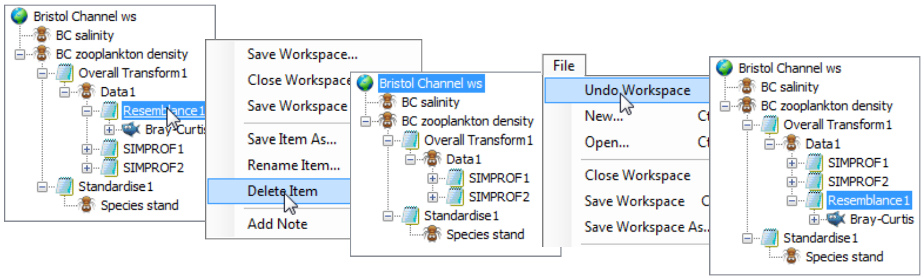
Met briefly in Section 1 and again above, renaming or deleting windows in the Explorer tree is an essential part of keeping a workspace navigable and understandable, especially since workspaces for many real analyses can become voluminous! Renaming is accomplished in one of three ways: as mentioned above, by clicking twice (slowly) on the entry name and typing directly into its box; by taking File>Rename Data (this changes to Rename Results, Rename Resem etc., depending on the entry type); or by right-clicking when over the Explorer tree to obtain a ‘floating’ menu which includes a general Rename Item operation. If part of an analysis is wrong or unhelpful, and you wish to delete it altogether from the workspace, a similar pair of options exists: click on the results name or icon and take File>Delete Results, or from the floating (right-click) menu take Delete Item. This results window, and all items below it on the same branch (its derived windows) will be erased from the workspace. You are prompted with the entry name to make sure that this really is the window (and derived windows) that you want to delete.
Note that in PRIMER 7 such a deletion is now a reversible operation, with File>Undo Workspace, which can be operated repeatedly to back-track through many successive Delete and/or Rename steps on the File> menu (though not, of course, Save, Close, New or Open operations since they are either easily back-tracked in other ways or are patently irreversible – such as saving to external files, or closing a workspace and ignoring the warning to save it first). You might like to try this out on the current Bristol Channel zooplankton workspace (save it first before you experiment!). Note what happens on reinstatement of branches or terminal windows (often plots) after deletion: they are added back, as might be expected, to the end of the stack of items at the same branch level, rather than the precise position from which they were removed (of course they retain exactly the same hierarchical position in the Explorer tree structure). One by-product of repeated deletion and reinstatement could thus be a limited ability to re-arrange the main strands of an analysis or the order of duplicated plots (e.g. a range of bubble plots, see next section) within the Explorer tree.
Saving plots
The name of a window can also be changed as part of the process of saving it, as a file external to the workspace: if the file is given a different name in the act of saving it, then that new name will also replace the existing entry in the Explorer tree. However, there is not the same need to save an individual data sheet, resemblance matrix, plot etc., that there was in the early versions of PRIMER (e.g. v5) because, as we have seen many times now, the full workspace can be saved in a single Save Workspace As operation, and this is a convenient way to pass data analyses to other users of PRIMER, for example. Nonetheless, there may be occasions when data (or resemblance) matrices need to be saved in an export format, as Excel *.xls(x) or text format *.txt files, or in internal v7 or v6 binary format – note that the v6 and v7 binary data formats differ – with extensions *.pri (or *.sid), perhaps so that they can be opened in a different workspace. More commonly, individual windows which are saved externally to the software are likely to be plot files.
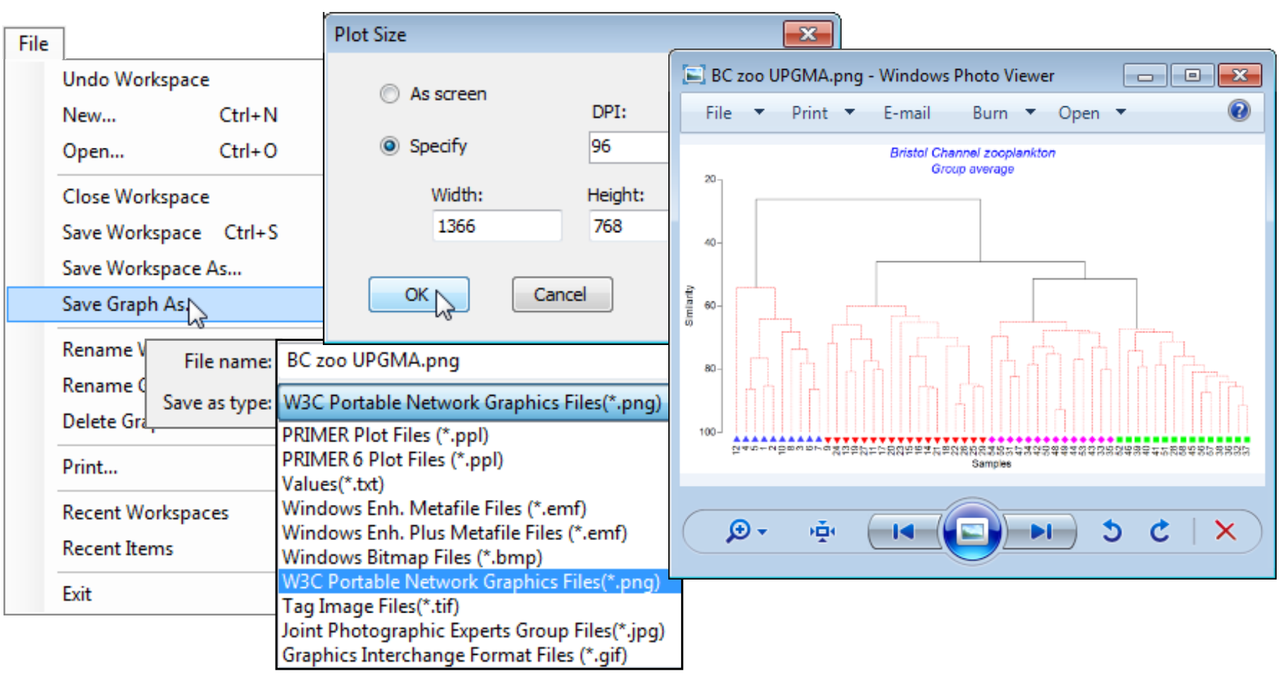
From the current Bristol Channel zooplankton workspace, try saving the dendrogram ![]() Graph3, for group average agglomerative clustering, by highlighting it in the Explorer tree and taking File> Save Graph As>(Filename: BC zoo UPGMA) & (Save as type: PRIMER Plot Files (.ppl)). This *.ppl extension denotes PRIMER 7’s internal binary format for graphics, and it too differs in v7 and v6 – if a v6 format plot file is required (for those plot types existing in the earlier version) then it should be explicitly chosen by (Save as type: PRIMER 6 Plot Files (.ppl)). The main use of *.ppl format files is likely to be in passing plots to other PRIMER users, so note that, whilst PRIMER 7 will read the v6 *.ppl format (forward compatibility), PRIMER 6 will not read v7 *.ppl files (no backward compatibility), hence the need to save explicitly in v6 format, on the rare occasion where this might be required. (Neither format can be accessed by any other software – even PRIMER v5). Demonstrate such transfer by launching a parallel run of PRIMER 7 (e.g. on the Windows 7 or 8 desktop, double-click on the
Graph3, for group average agglomerative clustering, by highlighting it in the Explorer tree and taking File> Save Graph As>(Filename: BC zoo UPGMA) & (Save as type: PRIMER Plot Files (.ppl)). This *.ppl extension denotes PRIMER 7’s internal binary format for graphics, and it too differs in v7 and v6 – if a v6 format plot file is required (for those plot types existing in the earlier version) then it should be explicitly chosen by (Save as type: PRIMER 6 Plot Files (.ppl)). The main use of *.ppl format files is likely to be in passing plots to other PRIMER users, so note that, whilst PRIMER 7 will read the v6 *.ppl format (forward compatibility), PRIMER 6 will not read v7 *.ppl files (no backward compatibility), hence the need to save explicitly in v6 format, on the rare occasion where this might be required. (Neither format can be accessed by any other software – even PRIMER v5). Demonstrate such transfer by launching a parallel run of PRIMER 7 (e.g. on the Windows 7 or 8 desktop, double-click on the ![]() desktop icon or right-click on the task bar icon and select PRIMER 7 again), to generate a second PRIMER desktop with an empty workspace. Open this newly created plot file into it, with File>Open>(File name: BC zoo UPGMA). You will see that, in spite of the link to its original data and resemblance matrix being cut, the plot is complete in itself, and still capable of being modified. It even holds with it the background information on factors, inherited from the data file, so all the changes seen in Section 6 can be implemented: not just resizing, titling, suppressing the key or history box, zooming, condensing, rotating, etc., but also changing displayed symbols to a different factor. It is important to realise that any changes made here will in no way affect the same plot held in the first PRIMER workspace. There is no dynamic linking of any sort between different workspaces or between workspaces and files external to them; only an unlinked copy of any file is ever opened in, or saved from, PRIMER. It should also be emphasised that PRIMER 6 and PRIMER 7 can both be running at the same time and will not interfere with each other, so if both are installed you may wish to try saving the BC zoo UPGMA dendrogram again from v7, this time with (Save as type: PRIMER 6 Plot Files (.ppl)), and re-opening it in v6.
desktop icon or right-click on the task bar icon and select PRIMER 7 again), to generate a second PRIMER desktop with an empty workspace. Open this newly created plot file into it, with File>Open>(File name: BC zoo UPGMA). You will see that, in spite of the link to its original data and resemblance matrix being cut, the plot is complete in itself, and still capable of being modified. It even holds with it the background information on factors, inherited from the data file, so all the changes seen in Section 6 can be implemented: not just resizing, titling, suppressing the key or history box, zooming, condensing, rotating, etc., but also changing displayed symbols to a different factor. It is important to realise that any changes made here will in no way affect the same plot held in the first PRIMER workspace. There is no dynamic linking of any sort between different workspaces or between workspaces and files external to them; only an unlinked copy of any file is ever opened in, or saved from, PRIMER. It should also be emphasised that PRIMER 6 and PRIMER 7 can both be running at the same time and will not interfere with each other, so if both are installed you may wish to try saving the BC zoo UPGMA dendrogram again from v7, this time with (Save as type: PRIMER 6 Plot Files (.ppl)), and re-opening it in v6.
Vector vs. pixel plots
Closing the second PRIMER desktop and returning to the original Bristol Channel ws workspace, note the other options for saving a dendrogram or any plot file with File>Save Graph As>(Save as type: $\text{\hspace{3mm}}$ ). The vector format Windows Enhanced Metafile (*.emf) will usually be the best option for exporting graphics from PRIMER into other applications, for fine tuning of title or key placement etc., in graphics presentation software. We saw earlier that Edit>Copy, when the active window is a plot, takes this vector format to the Windows clipboard, from where it can be pasted, for example, into Powerpoint. When Ungrouped it will be converted to a Microsoft drawing object and the lines, symbols, text boxes etc. which make up all plots can be subsequently modified, as appropriate.
In contrast, the other static plot output options from PRIMER all produce bitmap (i.e. pixel-based) files: *.bmp, *.png, *.tif , *.jpg and *.gif formats. Subsequent modification options are then rather limited. However, if the plot can be put into a satisfactory finalised form using the manipulations available within PRIMER, then high-quality output is certainly possible through the bitmap route. Saving the plot in one of these formats allows specification of the resolution, e.g. (Plot Size•As screen) or (Plot Size•Specify), with specifications being, for example, (Width: 1024) & (Height: 768), which give width and height of the image in pixels, and also specification of dots per inch, e.g. (DPI: 96). These files will generally be much larger than for vector plots.
A new feature in PRIMER 7 is the ability to output some plots in dynamic form, in cases where this is appropriate, via video format *.mp4 or animated *.gif files. We shall see such graphs in the next section, e.g. in 2- or 3-d animations of MDS iterations, temporal patterns and rotated 3-d plots.
Saving graph values; Saving results
Certain graphs, such as MDS ordinations (Section 8) or Cluster dendrograms, can be validly rotated in an infinity of ways (effectively), after the results window is generated, perhaps to align them better with a previous run under different transformation or coefficient choice. The plot is always saved in its currently rotated state, naturally, but these will not then correspond to the co-ordinate positions of ordination points, for example, which are listed in the results window. In order to make available the current ordination co-ordinates, or in the case of a dendrogram the ordering of the samples on the x-axis under the current rotation, an option to Save Graph Values is provided. This can be run in two ways, by File>Save Graph As>(Save as type: Values (*.txt)) or more directly by File>Save Graph Values As. The end result in both cases is a text file containing either x,y or x,y,z co-ordinate points for an ordination (each point to a line and tab separated within a line), or a list of the current order of samples in the dendrogram (each sample label to a line).
When they are active, results windows can be saved in just the same way, e.g. on CLUSTER1, File>Save Results As>(File name: BC UPGMA res) & (Save as type: Rich Text Files (*.rtf)) will save the individual clustering steps and associated SIMPROF tests to a file in rich-text format. The latter preserves variations in font size and use of italics when viewing the results window in Word, for example. The alternative is to Save as type: Text Files (*.txt) which outputs all text in a fixed size Courier font. The decision as to which option to select depends mainly on whether the text file will then be viewed in Word (use *.rtf) or in a simple text editor such as Notepad (use *.txt).
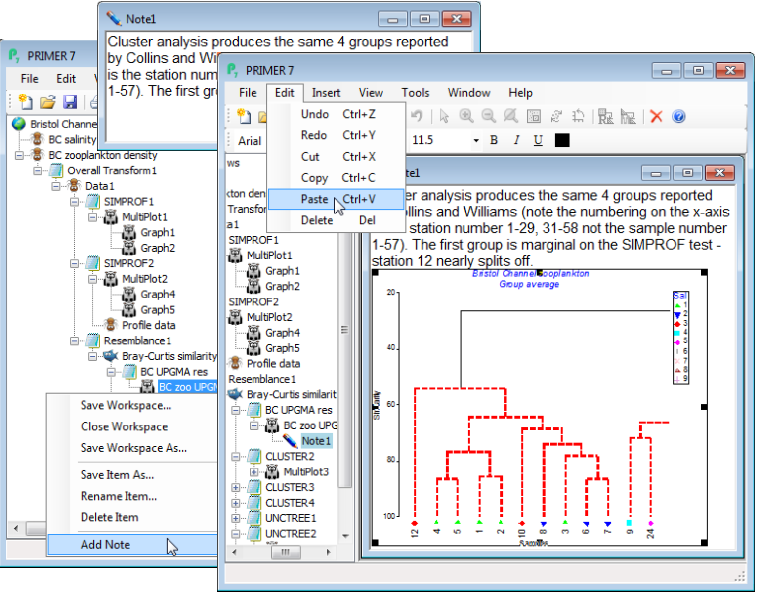
Adding notes
It is not permitted to edit directly the information in a results window. This tells you what operation or analysis was actually carried out, and what the outcome was, and should remain immutable, to avoid confusion if the workspace is revisited later. Naturally, you can highlight, then Edit>Copy (or Ctrl-C) results content to the Windows clipboard, and paste the information to an external text file, or Word or Excel file (tabular results from MDS, ANOSIM etc., see Sections 8 & 9, will map into appropriate Excel columns to allow simple editing and entry to other software – or indeed back into PRIMER). However, if you need to annotate the PRIMER session within the workspace, e.g. commenting on analysis steps or results, this can be achieved by Add Note, selected from the menu which appears when you right click on any item in the Explorer tree. A blank  Note window is opened for typing, and is displayed in the Explorer tree on a branch leading from the originally clicked item, which could just be the workspace name, in which case the Note will appear at the bottom of the tree – a convenient place to put ‘read-me’ information. Text can be pasted into the note via the clipboard (Edit>Paste or Ctrl-V), from outside or from elsewhere in the PRIMER session (e.g. from a results window or information copied from the Edit>Properties>Description box, etc.). You can even copy and paste whole graphs or highlighted portions of data sheets into a note window, so a note-form summary of the main features of the analysis can be held within the workspace (though lack of formatting usually makes this an intermediate step). Note windows can be renamed, deleted and saved, as with any other Explorer tree item, the save operation again involving a choice of *.txt or *.rtf formats (*.rtf is needed to preserve any plots in the output file).
Printing results and graphs
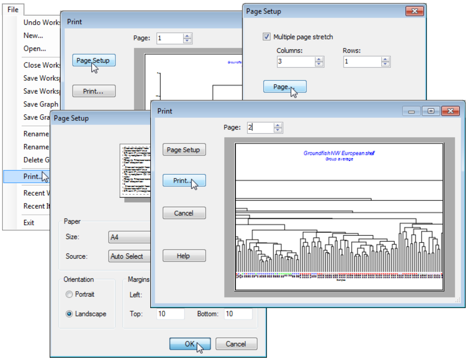
Direct printing from PRIMER is also possible for analysis endpoints such as results windows, all graphics windows, and notes (but not data sheets or resemblance matrices, which are generally too large and unwieldy for easy printing – selections of them are best saved to Excel or other software with capacity to size rows and columns into printable form). On plots, results or notes, File>Print>Print will take the default options and send you to the standard Windows dialog for selection of printer, any printer preferences, etc. However, for plots only, there is a PRIMER-specific option which can be taken prior to the final Print instruction, accessed by Page Setup after selection of File>Print. This allows a plot to be spread, horizontally and/or vertically, over multiple pages. It can sometimes be very useful in reading a cluster dendrogram based on many samples (thus printed over multiple horizontal pages) or in viewing a Shade Plot, perhaps from Wizards>Matrix display (Section 10), which can use a (✓Multiple page stretch) of the plot both horizontally and vertically. Also on the Page Setup dialog box, the Page button gives an alternative means of implementing simple printing choices of •Portrait or •Landscape, paper size and source, and margin sizes.
The facility to stretch a plot over multiple printed pages is best illustrated for one of the previous data sets so, leaving the Bristol Channel ws workspace open, launch another run of PRIMER and, if the workspace from the C:\Examples v7\Europe groundfish directory is available (last saved in Section 6), take File>Open>(File name: Groundfish ws) and click on the dendrogram, Graph2, to make that the active window – or re-run that cluster analysis of 277 samples. By File>Print>Page Setup>(✓Multiple page stretch)>(Columns: 3) & (Rows: 1)>Page>(Orientation: Landscape)>OK, the viewing window in the Print dialog box now shows the left side of the dendrogram as (Page: 1), and changing that to (Page: 2) displays the centre and (Page: 3) the right side, with some overlap to aid the physical pasting of the three printed pages which now result from Print. You will also find that an optimal printing will need to greatly reduce font and symbol sizes for all elements of the plot – in fact for most, if not all, of the font options (including Overall font scale) on the General, Titles, X axis, Y axis and Keys tabs of the Graph Options dialog and also the symbols plotted in the key, whose sizes are controlled from the (Size: $\text{\hspace{3mm}}$ ) option under Samp. labels & symbols.
File>Save Workspace the Groundfish ws and close down this second PRIMER desktop by the File>Exit menu item, leaving open the Bristol Channel ws workspace.
Automatic creation of multi-plots
The concept of a Multi-plot is a new feature in PRIMER 7. This construction has already been met in Section 4 where histograms of all selected environmental variables, using frequencies calculated over the samples, were presented in a single multi-plot window with component graphs consisting of the individual histograms for each variable (using Plots>Histogram Plot). You may have noted it again in the Explorer tree for the above Bristol Channel zooplankton analyses – see the PRIMER desktop in the first screen shot of this section – where a direct SIMPROF run (on one of the groups of samples identified by the cluster analysis) generated two plots: the similarity profiles, with their ‘expected’ limits under permutation, and the resulting histogram for the null distribution of the test statistic. Though these two plots are not of the same type (unlike the previous example of multiple histograms) it is natural to hold these related graphs together in a single construction, the multi-plot MultiPlot2. Another similar example is seen in this Bristol Channel ws workspace (MultiPlot3), of the dendrogram (Graph6) under flexible beta clustering, together with its associated line plot of the cophenetic correlation against the range of beta values (Graph7). PRIMER 7 now automatically packages such naturally related plot windows into a single multi-plot construction, essentially to neaten and simplify the ‘house-keeping’ of the Explorer tree rather than as a primary presentational tool – a multi-plot is often best thought of as a collection of thumb-nail graphs, each of which can (and should) always be viewed and manipulated individually by clicking anywhere over the space they occupy in the multi-plot window. In the Explorer tree the individual plot names are therefore all listed under the multi-plot name, e.g. Graph 4 and Graph5 under Multiplot2, and Graph6 and Graph7 under Multiplot3, etc., and it is often convenient to roll-up the individual plots by clicking on the rolled-out icon
![]() in front of the multi-plot name, which is then replaced by
in front of the multi-plot name, which is then replaced by
![]() , the rolled-up icon, with the individual plot names now hidden (but not, of course, deleted). This is particularly useful when large numbers of component plots are automatically created, as in the Histogram Plot on large numbers of variables, or in the next section, the new availability in PRIMER 7 of MDS plots in higher numbers of dimensions, with a run of Analyse>MDS>Non-metric MDS (nMDS)> (Min. dimension: 2) & (Max. dimension: 10) generating 9 ordination plots with their 9 associated Shepard diagrams, all automatically combined into an 18-component multi-plot (or 19 plots if the option is also taken to show the scree plot of stress vs. dimensionality). Of course, configurations in more than 3-dimensions can only be displayed by showing 3 axes at a time, but viewing the change in Shepard diagrams as dimensionality increases, in a single multi-plot, can be instructive.
, the rolled-up icon, with the individual plot names now hidden (but not, of course, deleted). This is particularly useful when large numbers of component plots are automatically created, as in the Histogram Plot on large numbers of variables, or in the next section, the new availability in PRIMER 7 of MDS plots in higher numbers of dimensions, with a run of Analyse>MDS>Non-metric MDS (nMDS)> (Min. dimension: 2) & (Max. dimension: 10) generating 9 ordination plots with their 9 associated Shepard diagrams, all automatically combined into an 18-component multi-plot (or 19 plots if the option is also taken to show the scree plot of stress vs. dimensionality). Of course, configurations in more than 3-dimensions can only be displayed by showing 3 axes at a time, but viewing the change in Shepard diagrams as dimensionality increases, in a single multi-plot, can be instructive.
User creation/ manipulation of multi-plots
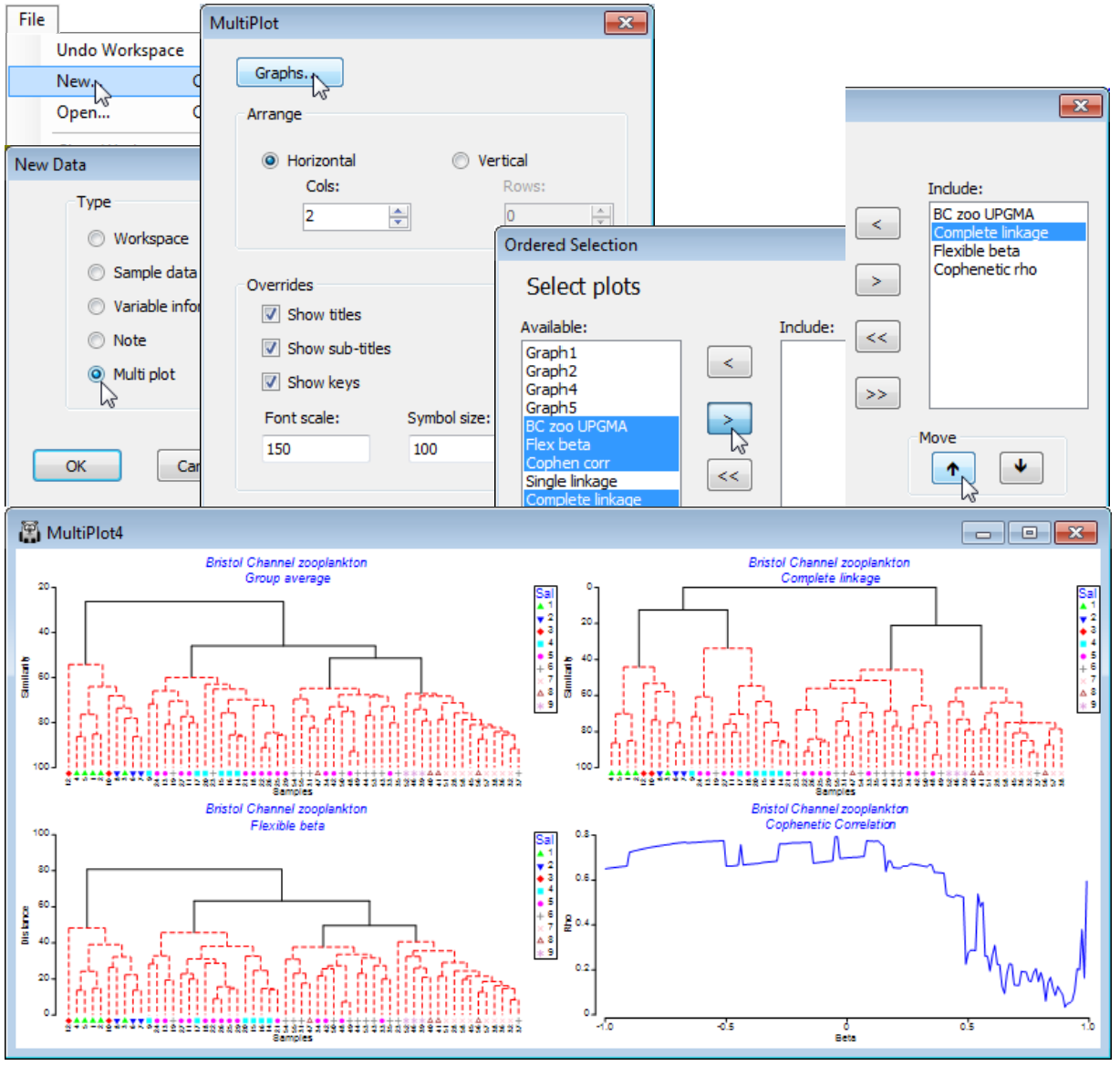
In addition to automatic generation by certain routines, multi-plots can be created and populated by the user, to hold sets of related plots in a single composite window. File>New>(•Multi plot) gives a dialog box headed by a Graphs button which allows an ordered selection from the windows for most of the single plot types in the workspace (for a contiguous set from the Available list, click on the first and last name whilst holding down the Shift key, or for a non-contiguous set, on individual names whilst holding down the Ctrl key, in standard Windows fashion). Then move them to the Include list with  and re-order them in the required sequence with the
  and
and  arrows. This sequence is followed either in horizontal rows or vertical columns with the choice of arrangement being chosen in the Multiplot dialog box. Given that the component plots can be of different types, the options for global change of features applying to all plots is inevitably limited. However, this dialog box – which can also be returned to from a completed multi-plot using Graph>Special – does allow for global setting of overall font and symbol sizes (where not limited to fit sample axes, as in the example below) and global suppression of main titles, sub-titles and keys. Clicking on individual plots in the multi-plot returns the active window to that specific graph, allowing the usual full range of changes to be made to all its properties. When this window is closed ( ), the multi-plot is again the active window and incorporates those changes (unless globally overridden).
The workspace Bristol Channel ws from C:\Examples v7\BC zooplankton should still be open, and it would be advisable to change the various dendrogram plot windows to more recognisable names, reflecting the different linkage methods, e.g. Complete linkage or Flexible beta (the linkage method can be found in the results window above each plot). Create a multi-plot with File>New>(•Multi plot)>(Arrange•Horizontal>Cols: 2) & (Font scale: 150) & Graphs, including the group average (UPGMA), complete and flexible beta dendrograms and the latter’s cophenetic plot, in that order. The plots will be placed in a 2-column stack (thus of 2 rows), with the order reading horizontally.
Plots menu
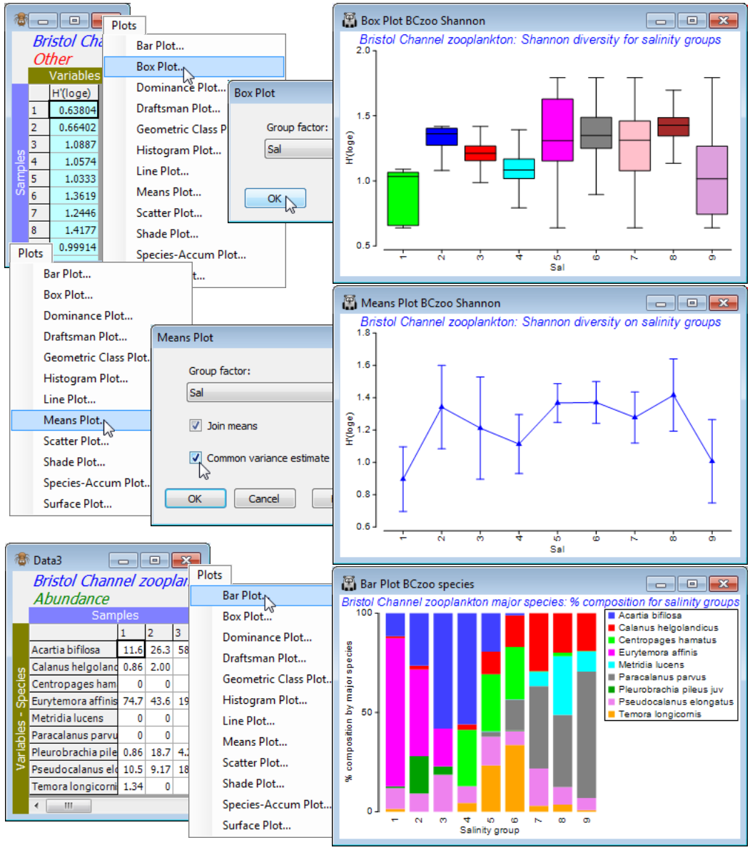
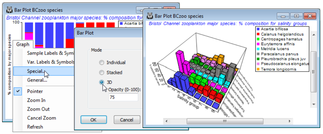
PRIMER 7 has a new Plots main menu, available when the active window is a data matrix. This brings together a number of standard plot formats, and more specialised ones, relevant to a range of multivariate analyses. Some are similar or identical to those in PRIMER 6, e.g. Plots>Dominance Plot, Geometric Class Plot and Species-Accum Plot (Section 16), and Draftsman Plot (already seen in Section 4 and again in Section 13). Others are new to PRIMER 7: the Histogram Plot was seen earlier (Section 4), as were Scatter Plot (Section 5) and Surface Plot (end of Section 4 and in Section 5). A significant new feature in PRIMER 7, the specialised Shade Plot, was introduced in Section 4 as a means to aid pre-treatment choice and is discussed in more detail in Section 10, in the context of interpreting species patterns across samples. There is a similar context for Line Plot, in the form of a multi-plot created by Wizards>Coherence plots, seen in Section 10, and the other three plot types in this menu are also standard graphic constructions: a Bar Plot can show relative composition of different species in each of a set of (averaged) samples, and Box Plot and Means Plot (Section 15) provide standard univariate tools pre- and post-hypothesis testing for a one-way layout, e.g. the latter giving confidence intervals for effect sizes (generalised to multivariate data by the bootstrap region plots of Section 17, under Analyse>Bootstrap Averages on resemblances).
Save and close the Bristol Channel workspace, Bristol Channel ws.
Workspace planning
To conclude this section, it is worth remarking that care taken in structuring workspaces will often pay dividends if the analysis results need to be returned to later. An Explorer tree represents a single workspace. It can contain several starting data matrices, the properties (factors etc.) of each being accessible to the others if they are based on an overlapping set of identical sample labels. (As seen previously, factors or indicators associated with a particular data matrix are automatically available to other sheets on the same branch, and on different branches by using the Factors> Import button). Such is the power and reach of PRIMER to quickly generate many plot and results windows that the user will probably find it a constant battle to keep workspaces down to a manageable size, both from the viewpoint of ease of navigation around them and of the size of a workspace file that needs to be transmitted to others (we have repeatedly seen the convenience of saving all the information in the workspace in a single file with a File>Save Workspace As step).
Firstly, it makes obvious sense to keep analyses on different studies in different workspaces but, also, analyses on different components of a single study may sometimes be better carried out in separate workspaces. The key criterion for using a single workspace is whether two data sets are to be combined or input to an analysis step together (e.g. species and matching environmental arrays), even if this is just as component parts of a single multi-plot. If not, they are probably best held and saved as separate workspaces. Multiple launches of the PRIMER desktop are straightforward, each with a different workspace (if the same workspace is opened twice – which is perfectly possible though should usually be avoided because of the likelihood of confusion when saving! – the second will be a copy of the saved version of the first workspace). Parallel desktops will not interfere with each other, and are never linked in any way. The only means of transfer between them is by saving individual sheets (e.g. data as *.pri) and then opening (a copy) of that file into the other workspace.
Secondly, ‘housekeeping’ within a workspace is important for intelligibility: key sheets of data, resemblances, results or plots – anything that needs to be selected as the active sheet for a further analysis, or a result or plot window that has been copied and saved to an outside presentation or manuscript – should be renamed in a meaningful way (all names in the Explorer tree need to differ, though PRIMER will ensure this by adding (2), (3), .. to the end of any name you supply which is already used in the workspace). Also, it is usually advisable to delete clutter, e.g. analyses you now realise were flawed or sub-optimal, using File>Delete … or Delete Item on the right-click menu when the window to be deleted is highlighted (branch entries below that will be deleted too). Use File>Undo Workspace if you make a mistake and want the excised portion back again! If you decide the sub-optimal analysis needs to stay in, as a reminder, then roll-up that particular branch (with ![]() ) and attach a note to the window above the
) and attach a note to the window above the ![]() icon, with right-click Add Note. In fact, it is desirable to make good use of this annotation feature more generally, to aid navigation.
icon, with right-click Add Note. In fact, it is desirable to make good use of this annotation feature more generally, to aid navigation.
Finally, some studies are sufficiently extensive, with data accreting over time, that it is advisable to resave the workspace with a modified name from time to time, so that at least an earlier version can be returned to should a disaster happen to the current workspace! Or it might be efficient to save the current data matrix (or matrices) in PRIMER binary format, *.pri, thus retaining all existing factors and indicators, and re-open this in a clear workspace for the next phase of the analysis.