9. Analysis of Similarity tests (unordered and ordered ANOSIM)
- ANOSIM introduction
- 1-way layout (WA fish diet example)
- Pairwise comparisons
- Other 1-way ANOSIM options
- 1-way layout (Biomarkers example)
- 1-way ordered ANOSIM (Ekofisk oil-field study)
- 2-way crossed ANOSIM (Tasmanian crabs study)
- 2-way crossed ANOSIM (Danish sediment data; Phuket coral reefs)
- 1-way ordered without replication
- 2-way crossed ordered test
- ANOSIM for 2-way crossed design with no replication (Exe study)
- 2-way nested ANOSIM (Calafuria macroalgae)
- 3-way crossed ANOSIM (King Wrasse diets)
- 3-way fully nested design (NZ holdfast fauna)
- 3-way crossed /nested design (Tees Bay macrofauna)
ANOSIM introduction
The series of ANOSIM (analysis of similarity) tests, accessed through Analyse>ANOSIM, operate on a resemblance matrix as the active sheet and carry out non-parametric tests for designs which broadly parallel univariate 1- and 2- way ANOVA (analysis of variance) crossed and nested cases, extended in PRIMER 7 to cover all combinations of crossed and nested 3-way designs. At the simplest level, a one-way layout of groups (e.g. of different times or sites or treatments), with replicates within each group, allows a test of the null hypothesis that there are no assemblage differences between the groups against an alternative which specifies that there are – but makes no assumption about the nature of those differences. However, another new feature in PRIMER 7 is the addition of a test of the same null hypothesis but against an alternative which specifies that the groups differ in a predetermined order, for example exhibiting a serial time trend or a continuous community change on approaching a point source impact. These ordered ANOSIM tests generalise, in a very natural way, the standard one-way ANOSIM R statistic to R$^\text{O}$ (superscript O for Ordered), defined in Chapter 6 of CiMC, and such ordering can be specified for all or any combination of factors in the 2- and 3-way designs. By narrowing the scope of the alternative hypothesis that the null is tested against, a greater degree of sensitivity (power) is obtained – though at the price of little or no sensitivity to detect group differences which do not conform to the hypothesised serial pattern. A crucial point to make is that the group designations (and specification of the group order under the alternative hypothesis) are made prior to seeing the data. ANOSIM is not a valid test of differences between groups generated by a cluster analysis, or other inspection of the data, other-wise the argument becomes entirely circular – use SIMPROF for these latter situations.
The simple 1-way R statistic is readily extended to a 2-way crossed layout, for example testing the null hypothesis that there are no differences between treatments (factor A), allowing for the fact that there may be site differences (factor B), in a case where all treatments are replicated at each site. Two-way crossed designs (A$\times$B) are symmetric, so the procedure can be reversed to give also a test for the hypothesis of no site differences given that there may be treatment differences – the routine gives both sets of tests automatically. The other 2-way option is a 2-way nested design, where the two factors are hierarchical, B(A), for example a top-level factor of treatment differences A (control vs impacted areas), with a second factor of different sites B within each treatment, and representative replicate samples from each site. A test can be carried out for significant differences between sites within a treatment, but at the next hierarchical level up, the primary interest would be in testing for assemblage differences due to treatment. This compares treatment differences against assemblage variation among sites within a treatment, rather than among the sample replicates at a site, and there is an example of this in Chapter 6, CiMC. A different style of test is required in the case of a 2- (or 3-)way crossed layout when there are no replicates (or no genuine replicates and it is wise to average the pseudo-replicates for each of the factor combinations). PRIMER 7 will automatically recognise situations in which replicates are not available and attempt to calculate a different test statistic $\rho$ (in whatever combinations of 2- and 3-factor designs it is encountered).
Three-way crossed and nested designs, also now covered in PRIMER 7, are of the types: A$\times$B$\times$C, fully crossed; C(B(A)), fully nested, C within B within A; C(A$\times$B), C nested in all combinations of A crossed with B; and B$\times$C(A), B crossed with C, where C is nested in A. These routines are all permutation tests, making a bare minimum of assumptions and consistent with the philosophy of the PRIMER routines that the primary information on relationships among samples is summarised in the ranks of the resemblance matrix – the basis for the preferred ordination technique of non-metric MDS. The tests apply to any resemblance matrix, so are equally effective at testing for assemblage change on biotic similarities, environmental change on Euclidean or other distances, change in biomarkers, particle sizes etc. None of the construction or concepts underpinning these tests is covered in this Section – that is all in the extensive Chapter 6 of CiMC, which includes the detailed Tables 6.3 and 6.4, listing the precise test statistics (and whether pairwise tests are possible when there are more than two levels of a factor) for every combination of: 1-, 2- and 3-way tests; unordered or ordered alternative hypotheses; and with or without replication. (That chapter finishes with some comments on the limits of construction of purely non-parametric tests, e.g. the non-existence of tests for interaction – a metric concept and the springboard for PERMANOVA). The below simply shows examples of the different tests and how the results windows are interpreted.
1-way layout (WA fish diet example)
Return to the W Australian fish diet data, introduced at the start of Section 4 and last seen under the Higher-d & scree plots heading of Section 8, showing MDS plots of dietary categories found in 65 (pooled) gut samples from 7 fish species. If the workspace WA fish ws is not available, re-open the data WA fish diets %vol.pri in C:\Examples v7\WA fish diets, exclude the samples A9, B3 and B4 (justifiable on the grounds of very low total gut content), standardise the samples, transform them with square root and take Bray-Curtis similarities, renaming this WA B-C sim. Re-run the nMDS and note that the number of replicates – the pools of fish from each species – is very uneven (from 3 to 15), as is the variability in diet for the different species (the dispersion of samples in the MDS space). Assumptions of balanced replication and the equivalent of ANOVA variance homogeneity are clearly not met here, but the ANOSIM test does not require such assumptions for its validity. Approximate balance in replication is still a good idea because it enhances the sensitivity of the tests, and comparable multivariate dispersion within each group makes interpretation simpler, but neither is possible here. ANOSIM tests the hypothesis that there are no dietary differences of any sort among the fish species. This null hypothesis can be rejected either because species require different food sources or because some have a much more variable diets than others, though they may feed on some of the same items – either or both reasons may contribute to rejection of the null.
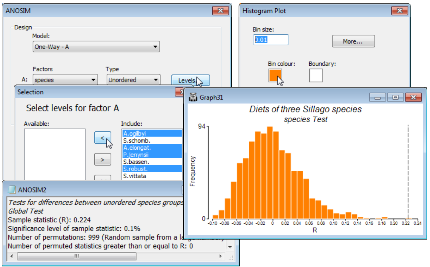
From the active window WA B-C sim, take Analyse>ANOSIM>(Model•One-Way - A)>(Factors A: species)>(Type Unordered), since clearly there is no prior expectation that if the diets differ then they can only do so along a steady gradient of change in a particular order of the fish species. (This is, however, exactly the expectation we have later when looking at the dietary changes of a single fish species at different stages of maturity, when the logical test will be an Ordered one). On the other choices, take (✓Pairwise tests R to worksheet) but leave the default settings for the remaining options, e.g. (Max permutations: 999) and Levels specifies that all 7 fish species are to be included. Three windows are created in the Explorer tree. ANOSIM1 is the results window, specifying the sheet and factor on which the test is performed, and giving the results of the overall ANOSIM test of the hypothesis of no differences in diet among any of the fish species, followed (when there are more than two groups, as here) by pairwise tests between the diets of every pair of fish species. The second output is a histogram of the permutation distribution of the ANOSIM test statistic, R, under the null hypothesis of the global test (though note that it is not the correct permutation distribution for any of the pairwise tests). The third output, requested here, is the set of observed pairwise R values held as a triangular (resemblance) matrix, and a similar option exists (not taken) to place the % significance levels for this set of pairwise tests in a further resemblance matrix.
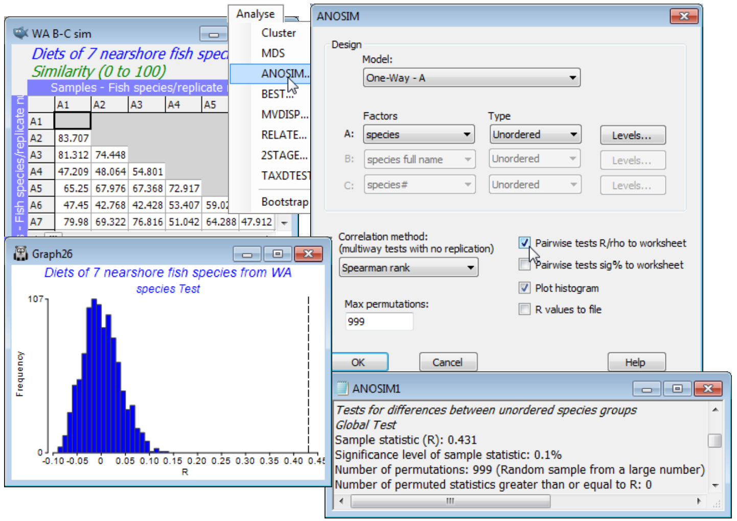
This histogram is centred around zero – if there are no dietary differences then the average rank resemblance among and within groups will be much the same, and R (based on the difference between these two averages, see Chapter 6, CiMC) will be near zero. It can rise a little above (or below) zero by chance, when there are no differences among diets, but the histogram shows that it will never get larger than about R = 0.15. The true value of R for these data is also shown, as a dotted line, namely R = 0.43, and this is clearly much larger than any of the 999 permuted values, causing rejection of the null hypothesis at a significance level of at least 1 in 1000 (P<0.001, or as the PRIMER output prefers it: p<0.1%). The same information is repeated in the results window ANOSIM1 under the heading Global Test, namely the overall observed R statistic of 0.431, its significance level (p<0.1%), how many permutations were computed in order to determine this (999), and how many of those permutations gave an R value as large, or larger, than the observed R of 0.431 (none). The total number of possible permutations – distinct ways of dividing the 65 samples amongst the 7 fish species, keeping the same number of replicates for each species – is extremely large and is therefore not displayed. In other cases, with few replicates, this third row will give the exact number of possible permutations, and if this is less than the specified (Max permutations: ) in the ANOSIM dialog box, then R will be evaluated for all possible permutations. Setting (Max permutations: 9999) will increase the significance level here to p<0.01% (it is clear from the histogram that, almost irrespective of how many permutations are chosen, a value as large as R = 0.43 will not be obtained by chance, so the significance level for the global test of no dietary differences can be made arbitrarily small, by increasing the number of permutations).
Pairwise comparisons
The table ending the results window gives the pairwise comparisons. For each pair of groups (fish species), the first data column is of pairwise R statistics. These are again a difference of average rank dissimilarities between and within the two groups, scaled so that R varies between roughly 0: there are no differences, and 1: all dissimilarities between gut contents of different fish species are larger than any dissimilarity among samples within either species. The second column gives the statistical significance for a test of R = 0 (again as a percentage, so that p<0.1% means less than a 1 in 1000 chance). The number of possible permutations follows, then the number actually computed – 999 in most cases because the possible number is usually much larger than this, here. The final column gives the number of R values from the permutations that exceed (or equal) the real R in the first column, from which the significance in column 2 is calculated. [Note that there needs to be a slight difference in this computation depending on whether all possible permutations are evaluated. Thus row 1: A. ogilbyi v S. schomb., R = 0.868, p<100(1+0)/(1+999) = 0.1%, whereas row 12: A. elongat. v P. jenynsii, R = 0.919, p = 100(1/126) = 0.8%. The second is clearest: the observed value of 0.919 is the most extreme of 126 permutations and thus has probability 1 in 126 of occurring by chance. In the first case, we do not observe the real value of 0.868 in our randomly chosen set of 999 permutations, but that does not make the probability p = 0/999 = 0. We know there exists one permutation which would give R at least 0.868 – the real configuration – and we have looked at 1000 permutations overall (the 999 random plus the real one) so the probability is < 1 in 1000.]
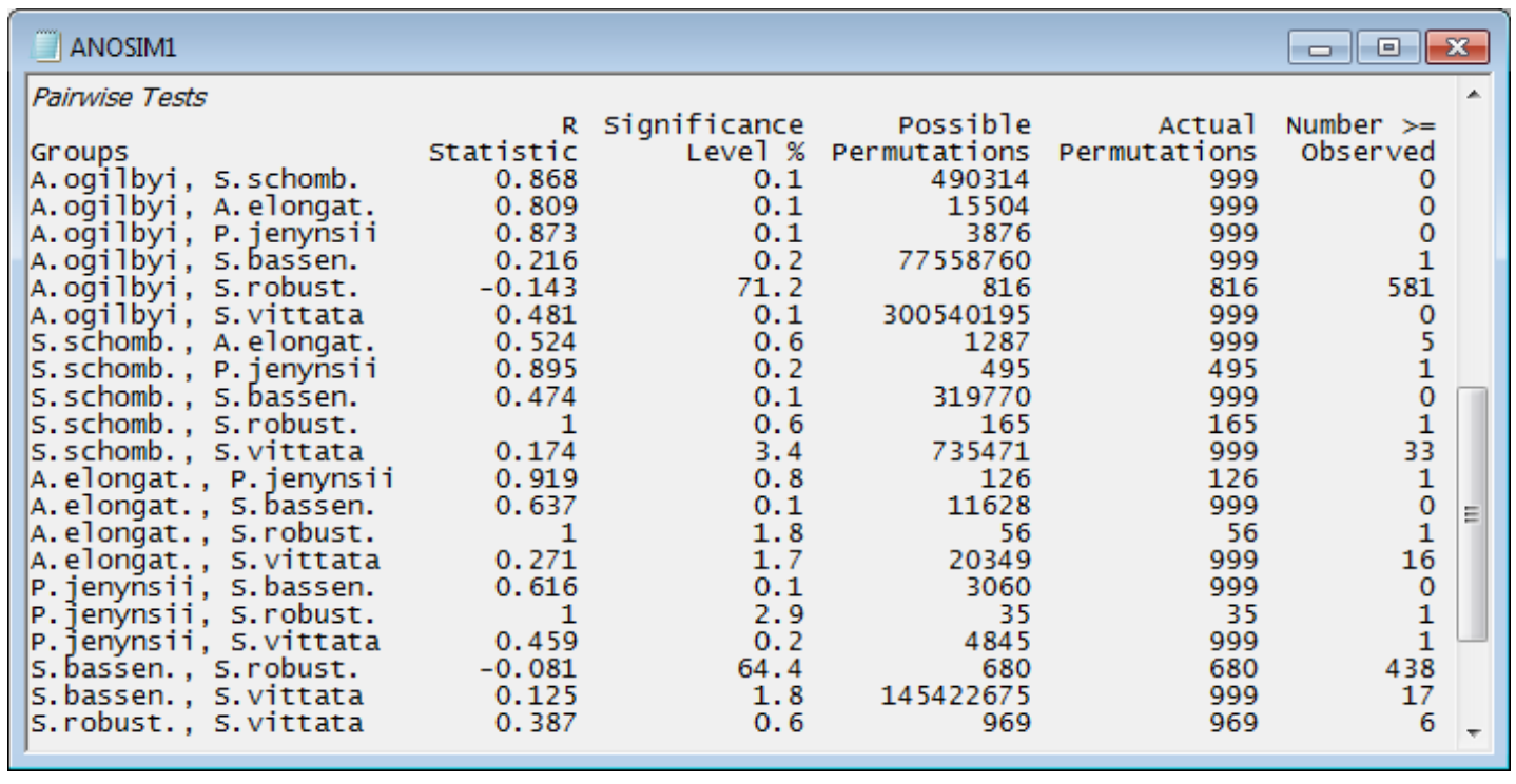
Interpreting these pairwise tables must be done with care. The significance level is very dependent on the number of replicates in the comparison. For example, row 4: A. ogilbyi v S. bassen., p<0.2% (your value may differ slightly because each time the routine is run, different random permutations will be generated). This appears highly significant, but the R value is negligibly small, at 0.216. The test tells us that these two species probably do not have exactly the same diet (the hypothesis R = 0 can be rejected) but the R value tells us that the diets are strongly overlapping and barely differ (R is close to zero). This can happen, just as in ordinary univariate statistics, because the number of replicates is large for the two groups, giving 77 million possible permutations – biologically trivial differences can still be statistically significant when the test’s power is large. In total contrast, row 17: P. jenynsii v S. robust., p<2.9%, still significant but only just (at the 5% level), has an observed R of 1.0, the largest possible value, which shows completely different diets. Such a large value of R does not give a small value of p because there are only 35 possible permutations (few replicates in both groups). Which is therefore the most useful column to interpret? It has to be the R values and not the p values. R is largely not a function of the number of replicates (i.e. possible permutations) but an absolute measure of differences between two or more groups in the high-dimensional space of the data, whereas p is always hijacked by the sample size. It is for this reason that PRIMER does not implement a Bonferroni-type correction on its pairwise significance levels – it gives an illusion of certitude which is not justified. The global test of any differences between groups is important: if the null hypothesis is not rejected then the user has no licence to look at the pairwise comparisons. However, if the global test strongly suggests that there are differences worth examining, the focus shifts to the pairwise R values – large values there indicate where the major differences are found.
Other 1-way ANOSIM options
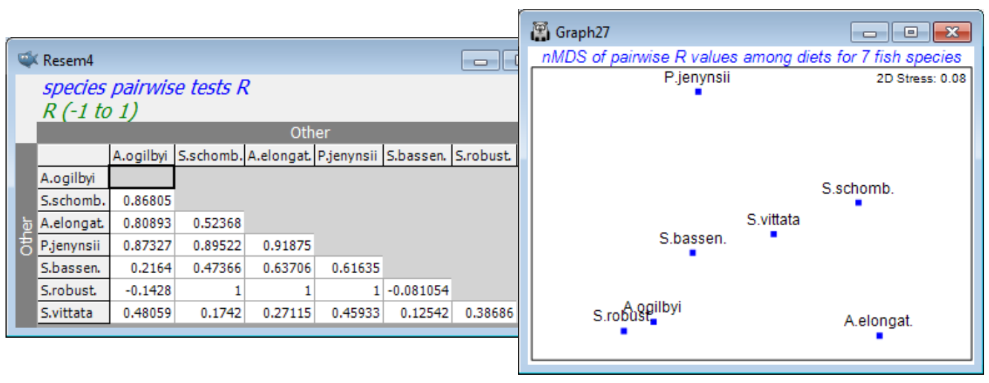
Checking the (✓Pairwise tests to worksheet) box has also sent the above R values to a worksheet in triangular format, which could be a useful layout for tabulating ANOSIM results in a publication. More subtly, this can be regarded as a resemblance matrix (of distance-type) in its own right – the higher the value of R the greater the separation of replicates from two groups in the high-d (prey) space. Inputting this to an MDS plot will display the relationships between these 7 groups, and can be seen as a type of means plot. [Note that this triangular array is not a sensible distance matrix at present because it can, and does, contain (small) negative values. Input to metric MDS without some prior rescaling would be problematic therefore. However, nMDS effectively works only on the rank orders of the entries so there is no need to rescale them – the lowest values (the negative ones) indicate the least established differences in diet and the highest values (R=1) the greatest differences, which is exactly what is required for a sensible nMDS plot here. Dropping the negative signs, by taking absolute values of the entries, would not be the technically correct approach here.]
The more straightforward means plots, as we have seen before, is to average the replicates, and then calculate Bray-Curtis between these mean dietary samples, ordinating by nMDS or mMDS. But there are many other possibilities for a direct means plot! The data could be transformed before or after averaging, or the dissimilarities could be averaged – or even their ranks averaged. PRIMER 7 now has the option to average (dis)similarities across a group structure, with Tools>Average for an active window of a resemblance matrix. Tools>Rank distance will also replace resemblance entries with their ranks. (A further option is given in the PERMANOVA+ add-on, of computing distances among centroids in the high-d PCO space formed from the resemblance matrix). These will all give means plots with slightly different emphases. In the case of the matrix of R values, this highlights relative group separations, i.e. adjusting differences by within-group dispersion.
Other options within the ANOSIM routine include the ability to manipulate the histogram for the global R statistic by rescaling axes, titles etc. (the usual Graph>Sample Labels & Symbols menu) and changing bin widths and, in v7, bin colours (Graph>Special), as for any other histogram plot. There is also a check box in the ANOSIM dialog to send (✓R values to file). You would then need to supply an *.txt file name which will hold a simple list – one number to a line, in simple text – of the R values for the 999 (or however many) permutations carried out for the global test. This would allow the null distribution data to be replotted, for example, in another statistical/graphical package.
As noted earlier, the plotted histogram (and the listed R values) refer only to the global test for no differences among any of the groups. If you require a histogram for a specific pairwise comparison then you will need to pick out that pair of groups and re-run ANOSIM, selecting either externally, by Select>Samples on the original resemblance matrix, or internally, using the Levels button for A on the ANOSIM dialog. Both lead to the usual Selection dialog. For a pairwise test, it will make no difference to the R value (or to its significance level) whether the results are read from the above pairwise table or recalculated with just those groups selected, so this would only be useful: a) if you required the pairwise histogram, or b) a test for a specific subset of three groups, four groups etc. was needed. As seen in Section 3, a relevant a priori hypothesis here concerns whether there are detectable dietary differences between the three congeneric Sillago fish species (S. schomburgkii, S. bassensis and S. vittata). After testing this, save and close the workspace WA fish ws.
1-way layout (Biomarkers example)
ANOSIM applies equally well to data on environmental, biomarker or morphometric variables, which might be transformable to approximate normality; it is then a robust alternative to classical multivariate (MANOVA) tests such as Wilks’ lambda. The inevitable slight loss in power of the non-parametric test, if the data really were multivariate normal (and had few enough variables in relation to sample sizes to allow proper estimation) is more than compensated for by its robustness, general applicability, and lack of assumptions such as constant variance-covariance structures.
Re open the N Sea ws workspace seen in Sections 4 & 5, with datasheet N Sea flounder biomarkers of 10 replicates from each of 5 N Sea sites, S3, S5, S6, S7, S9 (directory C:\Examples v7\N Sea biomarkers). Of the suite of 11 biomarkers it was previously suggested that EROD and LIPID VAC might benefit from square root transformation, being modestly right-skewed – earlier performed by highlighting them and Pre-treatment>Transformation(individual)>(Expression: SQR(V)). The variables are put on a common measurement scale with Pre-treatment>Normalise Variables and an appropriate resemblance calculation is Analyse>Resemblance>(Measure•Euclidean distance), before Analyse>ANOSIM on factor Site, as above. The results show a significant (mainly large) separation of the biomarker responses at all sites, seen clearly also in an nMDS plot (or mMDS would have nearly as good a stress here). Resave and close the workspace, N Sea ws.
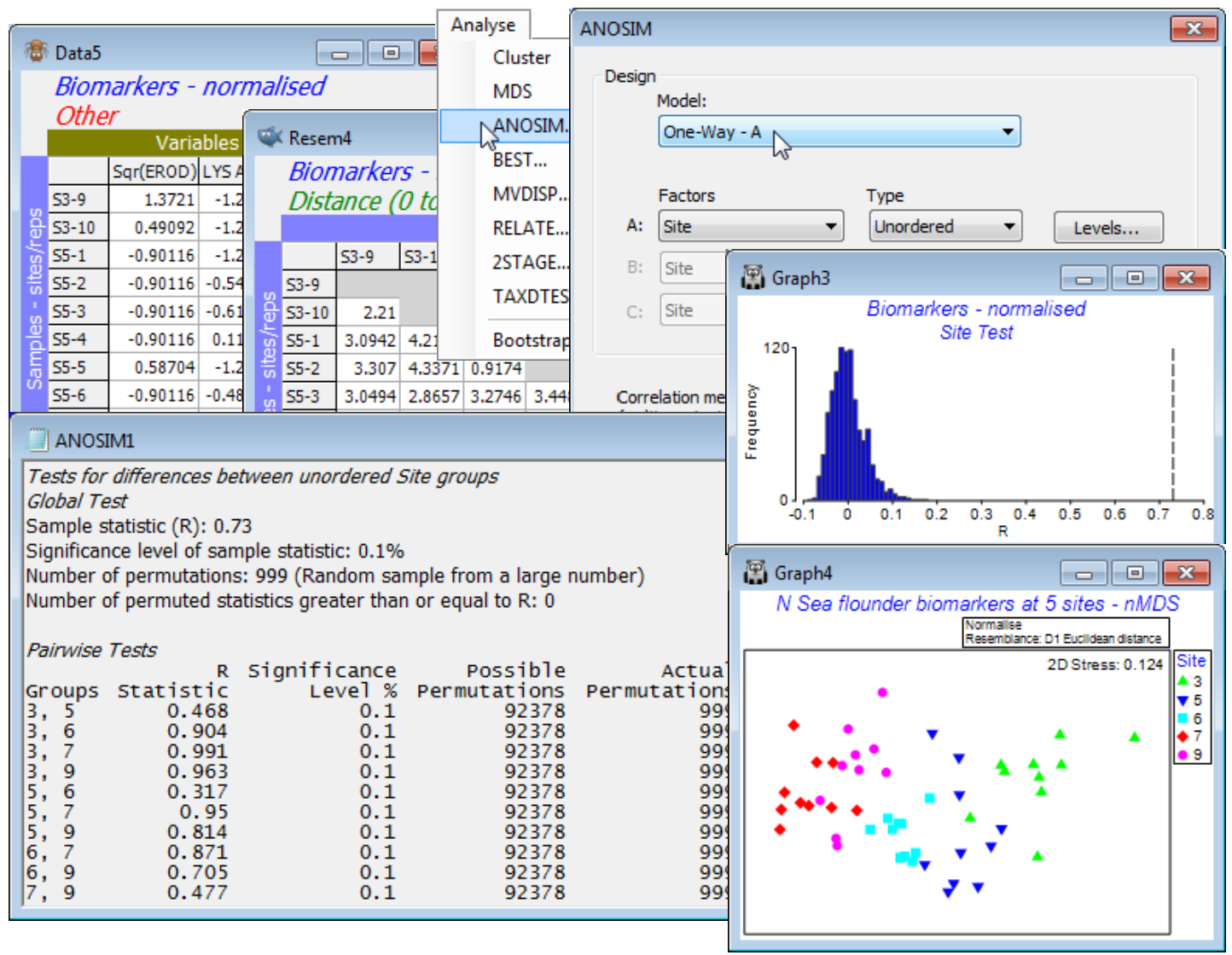
In this example, the sites were along a transect from the mouth of the Elbe (S3) to the Dogger Bank (S9) but there was no strong presumption in advance of the data collection that responses of the biomarker suite, if present at all, must conform to a monotonic gradient of change. This is not a clear case of a decreasing contaminant gradient with distance from a point source impact, since over such a large geographic region (and with motile organisms) many environmental drivers may be in play, only some of them anthropogenic. An ordered ANOSIM test would then run the risk of failing to detect differences among sites if these are not in the physical order of the sites along the transect. And, whilst the above nMDS does then show responses that are mainly aligned with the transect - and the ordered RO gives a similar and also highly significant value of 0.74 compared to the unordered R=0.73 statistic - this pattern is not entirely consistent (e.g. sites 6, 7 and 9). Of course, a decision about which test to use should be made prior to seeing any data, and it would have been unwise to opt for the ordered test and rule out any possibility of detecting community changes in which, for example, both ends of the transect were impacted in the same way (and therefore similar to each other) but the mid-transect sites reflected a different background state.
1-way ordered ANOSIM (Ekofisk oil-field study)
However, for the Ekofisk oil-field study of the last section there is a postulated cause for benthic community change (the presence of an oilfield) and impacts, if any, are expected to result in a monotonic change with increasing distance from the drilling centre. For the four distance groups, defined prior to the data analysis: D (<250m), C (250-1000m), B (1 - 3.5 km) and A (>3.5km), a test of the null hypothesis H$_0$:A=B=C=D against the ordered alternative H$_1$:A$\rightarrow$B$\rightarrow$C$\rightarrow$D (or vice-versa) is entirely appropriate, and inability to detect the above scenario (sites near and far from the rig being similar but intermediate sites differing) would usually be a price well worth paying in pursuit of a more powerful test of this specific (ordered) alternative hypothesis. [We return to this point, and example, in Section 14, based on the seriation with replication test of Somerfield PJ, Clarke KR & Olsgard F 2002, J Anim Ecol 71:581-593, which tackles the same problem with a slightly different (RELATE) statistic, $\rho$. The relationship of the new, ordered ANOSIM statistic to that for the previous Analyse>RELATE test is covered in Chapter 6 of CiMC].
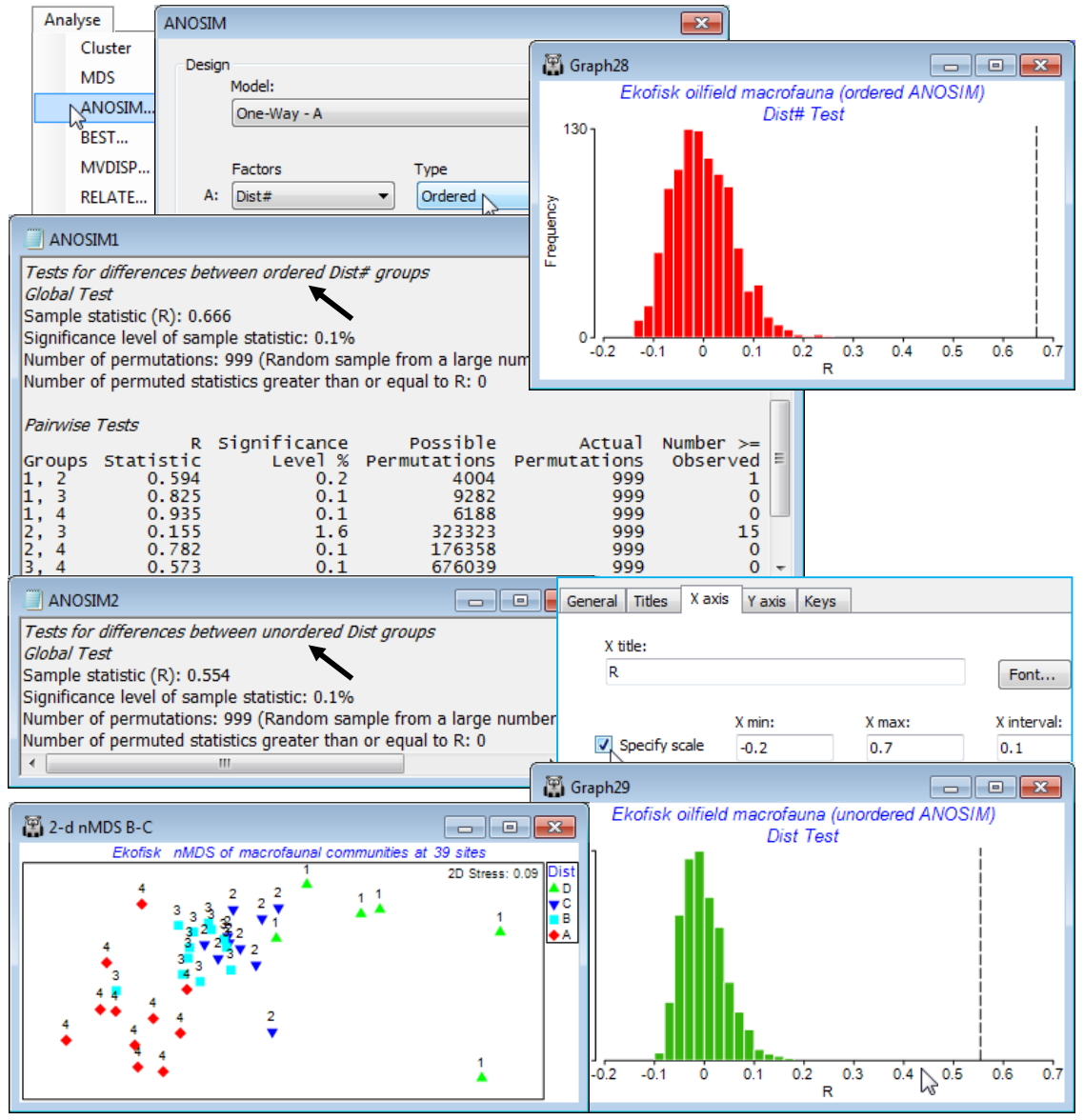
Re-open the Ekofisk ws workspace of Section 8, in which the data Ekofisk macrofauna counts from C:\Examples v7\Ekofisk macrofauna has been square-rooted and input to Bray-Curtis calculation, giving resemblance matrix B-C on sq rt. On this, take Analyse>ANOSIM>(Model•One-Way-A)> (Factors A: Dist#)>(Type Ordered). Note that the numeric form Dist# (levels 1-4) of the factor representing distances from the oilfield is required for the Ordered ANOSIM test; the alphabetic form Dist (levels D-A) is not recognised by PRIMER as an ordering (if Dist# is not available, re-create it by Edit>Factors>Add>(Add factor named: Dist#), and enter 1 at the top, opposite the first D, 2 opposite the first C, 3 when it changes to B, and 4 to A, then highlight the column and Fill>Value to fill in all the blanks appropriately).
The outcome is an ordered R$^\text{O}$ of 0.67 which, as can be seen from the null distribution histogram, unquestionably rejects the null hypothesis (R$^\text{O}$ = 0) on a p<0.1% level test (i.e. P<0.001), and would do so for massively smaller values of p. The ensuing pairwise tests show a clear pattern of increasing R for increasing separation of the distance groups, exactly as one would expect from a serial community change. Only the differences between groups 2 and 3 (C and B) are at all border-line, with a low R of 0.16 (but still significant in conventional terms, at the 2% level). Note that the pairwise tests are always ordinary R statistics – there is no difference between an ordered and an unordered test when there are only two groups! Now re-run the ANOSIM specifying the unordered case, this time using either the alphabetic or numeric factors Dist or Dist# (it no longer matters). The R = 0.55 value, though still massively significant, is seen to be lower than the R$^\text{O}$ = 0.67 of the ordered test. These statistics are directly comparable, and show the better fit of the underlying model (see Chapter 6, CiMC) of equi-stepped serial change than that of equi-different groups. This is clearly evident also from the previous nMDS plot. Save and close the workspace Ekofisk ws.
2-way crossed ANOSIM (Tasmanian crabs study)
An example of a 2-way crossed layout was introduced in Section 1, for meiofaunal communities in sediment patches either disturbed or undisturbed by soldier crabs (treatment factor Trt, levels D/U, factor A), over four areas of Tasmanian sandflat (block factor Blk, levels 1-4, factor B), with two replicates for each of the 8 combinations. Setting up of these factors was described in Section 2. Open (or create) the workspace Tasmania ws with datasheet Tasmania nematodes, take a fourth-root transform and compute Bray-Curtis similarity, renamed Nem B-C. Run this through nMDS and note the way the samples split rather convincingly between the effects of the different regions of sandflat (blocks, roughly across the page) and disturbed or undisturbed (treatments, roughly up the page; click on the Blk-Trt key to change symbol type/colour for blocks and open/closed for treatments). There are so few replicates, however, that this is not clear-cut and does need testing. Also, stress is quite high (about 0.16) so the picture may be misleading, and the test needs to be in the full-dimensional space represented by the resemblance matrix, as ANOSIM tests always are. Two-way crossed ANOSIM is carried out for the null hypotheses, H$_0$: no treatment effect, allowing for the fact that there may be differences between blocks, and also symmetrically for H$_0$: no block effect, allowing for the fact that there may be treatment effects. The test statistic for treatments is now the average of the 1-way ANOSIM R values for testing the treatments separately within each block, and the permutation procedure is also a constrained one, within blocks (see Chapter 6 and Fig. 6.7 of CiMC, which analyses the same study but for the full meiofaunal data – nematodes and copepods combined – for which the outcome is even clearer). Here, with Nem B-C as the active sheet, take Analyse>ANOSIM>(Model: Two-Way Crossed - AxB)>(Factors A: Trt & B: Blk) and both factors are treated as unordered (the treatment only has two levels anyway, and though the block areas will vary in their nematode assemblages there is no expectation that this will be on a strong gradient). Again, note that we could have restricted the analysis to use only some of the levels of either factor, with the Levels buttons, though this is not appropriate here.
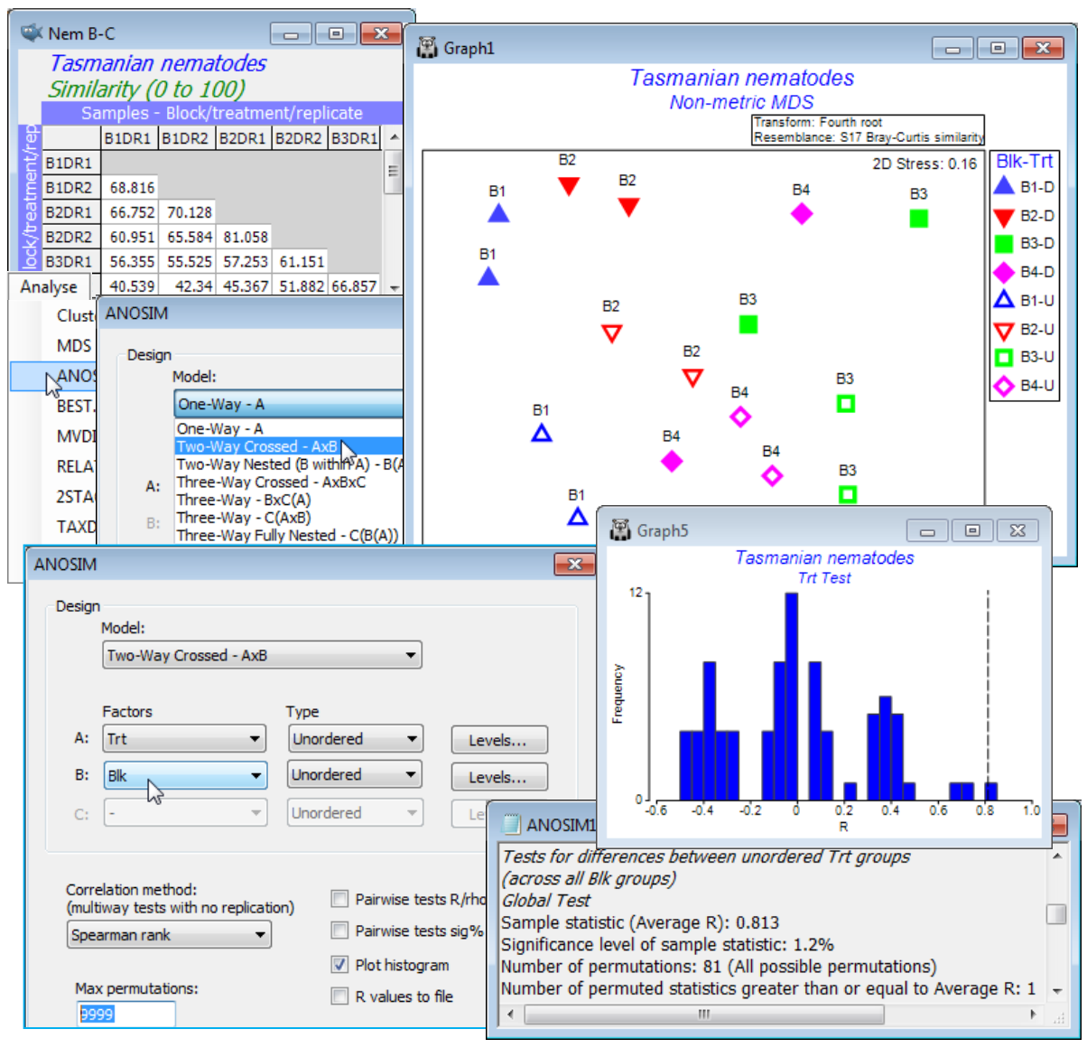
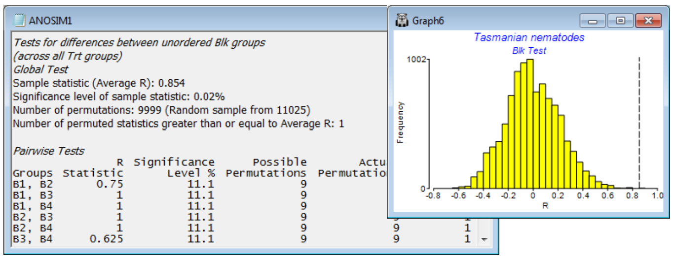
For the test of the treatment effect, the histogram shows a typical null distribution for the ANOSIM test statistic when there are few replicates. With only 81 distinct permutations permitted (these correspond to all ways of simultaneously exchanging the four replicates within each block), the range of values that the statistic can take when there is no treatment effect is not at all smooth. This demonstrates why the null permutation distribution has to be recreated for each new data set and cannot rely on standard tables or distributional forms. And clearly there is no point for this test in increasing to (Max permutations: 9999), as we have done here – there are only 81 permutations and ANOSIM does them all. Nonetheless, the results in ANOSIM1 show that the observed statistic for testing treatments (global R = 0.813) is the largest obtainable for the 81 permutations, so gives a significance level of 1 in 81 (p = 1.2%). This would normally be considered sufficient to cast doubt on the null hypothesis of no treatment effect. If there were more than two treatments, the global test would be followed by pairwise comparison of treatments, exactly as for the 1-way ANOSIM case.
The second plot is much smoother because there are 11025 possible permutations of the replicates across blocks within each treatment, corresponding to the null hypothesis of no block effect, and a random subset (with replacement) of most of them has been evaluated. In fact, having seen that there are only 11025 to find, it would make sense to repeat the analysis, setting (Max permutations: 12000) – or any number >11025 – because ANOSIM will then compute the full set of 11025. But this was not done here, and the observed average R of 0.854 was seen to be the most extreme of all but one of the 9999 permutations examined – almost certainly that one was the real configuration but we cannot guarantee that if not all the permutations are evaluated, so the significance level is a (slightly conservative) 2 in 10000, i.e. p<0.02%. There is little merit in then considering the pair-wise tests of Block1 v Block2, Block 1 v Block3 etc. The key thing to have established is that there are natural changes in the nematode assemblage across the sandflat, so that removing this block factor from the test for treatments was worthwhile (the nMDS shows that a 1-way design in which block-to-block changes become part of the replicate variability would largely fail to pull out the treatment effect). Individual block differences are not of interest, but if they were, the Pairwise Tests table in ANOSIM1 shows that all blocks are well separated from each other (all pairwise R values are large). Note that none of these pairwise comparisons has enough replicates (and thus permutations) to allow a sensible significance test. In all cases the observed configuration is the most extreme permutation, best separating the two blocks, but with only 9 permutations that gives significance of only p = 11.1%. It is not logical to conclude that there are no differences between any pair of blocks when the global test has just shown that there are massive and highly significant differences amongst all four blocks! As remarked for 1-way ANOSIM, the focus should be on showing significance of the global R (otherwise pairwise comparisons should not be pursued) and then the pairwise R values themselves, to see where the large effects are (here, between all pairs).
2-way crossed ANOSIM (Danish sediment data; Phuket coral reefs)
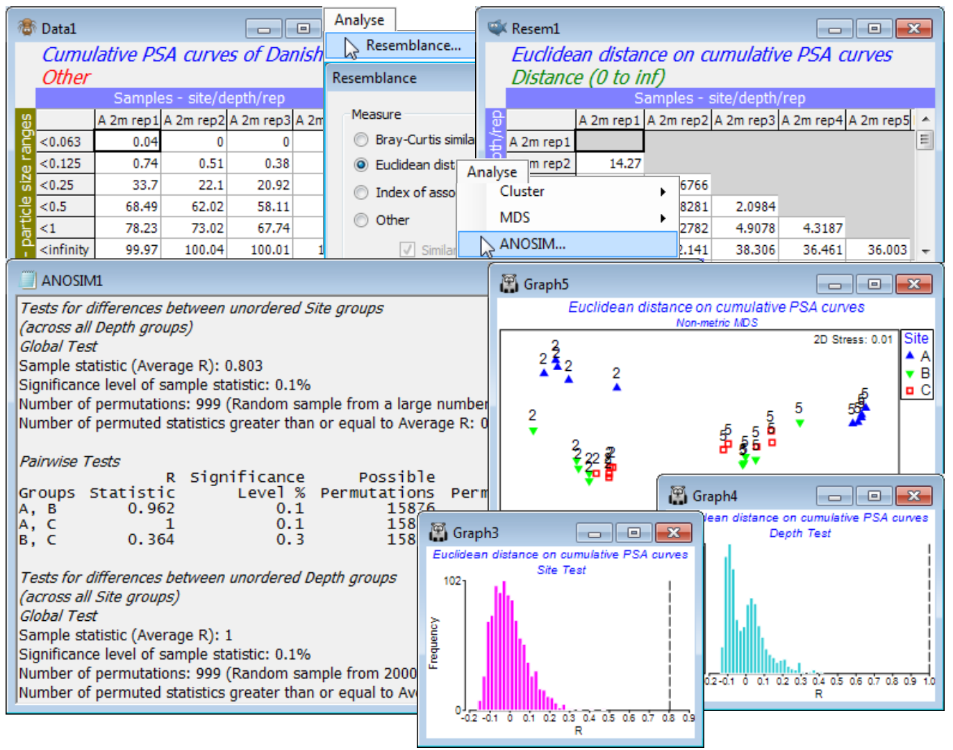
For an example of a 2-way crossed ANOSIM test in a very different context, save and close the above workspace and return to the particle size distributions from Danish sediments introduced at the very end of Section 4 – the workspace Denmark ws in C:\Examples v7\Denmark PSA, with particle size frequency data (over 6 size-categories) in Denmark PSA histogram, for 3 sites (A, B, C) crossed with 2 depths (2m and 5m), and 5 replicate samples from each combination of site and depth. A distance measure such as Euclidean (or Manhattan or Maximum distance, see Section 5) is appropriate for defining the resemblance between two distribution curves.
As suggested earlier, apply this to the (smoother) cumulative frequencies from Pre-treatment> Cumulate Samples>(Variable Order•As worksheet), and on the resulting resemblance matrix run Analyse>ANOSIM, with the 2-way crossed option for factors Site and Depth (in some cases, the latter might be considered ordered, but we have only 2 depths here so the distinction is irrelevant; Site is clearly unordered). The results show perfect separation of the depths (global average R = 1, p<0.1%) and strong separation of the sites (global average R = 0.80, p<0.1%). The large number of possible permutations means that these p values could be made almost arbitrarily small, as is clear from the null distribution histograms. Pairwise site tests show, however, that B and C are not well separated (average R = 0.36, though still larger than all but 2 of the 999 permutations considered from the full set of 15876, thus p<0.3%), as is also seen in an nMDS plot on the Euclidean distance matrix (or a PCA, see Section 12). Close this workspace – it will not be needed again.
The study of coral reef assemblages at Cape Panwa, Phuket, Thailand – introduced near the end of Section 8 – measured area cover of corals on twelve 10m line samples taken perpendicularly to an onshore to offshore transect (A), over a time series of years. The previous workspace, Phuket ws, contained the data only for 1983-87, and 1983 was selected to visualise community change along the A transect, seen in an nMDS. Here, you should open into that workspace (or a clear one) data from the 7 middle years, Phuket coral cover 88-97 in C:\Examples v7\Phuket corals. Factors Year (88, 91, 92, 93, 94, 95, 97) and Position on the A transect (1-12) form a 2-way crossed design, because each position is examined (plotless line sample) in each year, but there is no replication
1-way ordered without replication
In the unordered 1-way design, replication is essential for any sort of test (otherwise how can you tell whether single samples from groups A, B, C, … are from the same or different communities? – there are no within-group rank dissimilarities to compare with among-group ones). For the ordered 1-way design, however, the test statistic R$^\text{O}$ can still be constructed – see the explanation in CiMC Chapter 6 under ANOSIM for ordered factors, where the statistic for the unreplicated design is designated R$^\text{Os}$, for ordered single, rather than R$^\text{Oc}$, for ordered category (though in both cases it is fundamentally the same slope statistic R$^\text{O}$ from a regression of rank dissimilarities against modelled rank distances under the alternative hypothesis). A univariate analogue you may find it helpful to think about is testing whether differences in a variable y bear any relation to given values of x. If you are not prepared to make any assumptions about the form of the relationship (the alternative hypothesis just says the values of y differ with those of x in some way unspecified) then you must have replicates at each x value in order to construct an (ANOVA-type) test. If, however, you set out to examine the alternative hypothesis that the relationship between y and x is linear, then there is a perfectly viable test without any replication of x levels, i.e. whether the slope of a linear regression of y on x is significantly different from zero. And you may choose that linear regression test even when there are replicates at each x level. This is actually a very precise analogue of the difference between ordered R$^\text{O}$ (regression-type) and unordered R (ANOVA-type) ANOSIM tests.
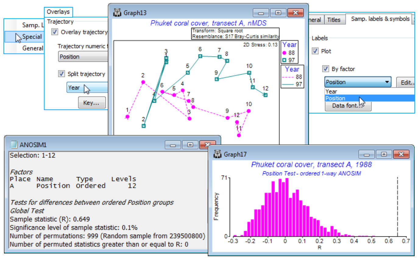
So, for the Phuket coral cover 88-97 data, take a square-root transform and Bray-Curtis similarities, selecting from the latter the first and last years 88 and 97 (i.e. 24 samples, the 12 transect positions in each year) and reproduce the nMDS plot seen in Fig. 6.14 of CiMC – with separate trajectories over transects for each year by taking Graph>Special>Overlays>(✓Overlay trajectory Position)> (✓Split trajectory Year) and on Samp. labels & symbols, (Labels✓Plot)>(✓By factor Position). It is scarcely necessary to test the null hypothesis of no Position effect for each of these years but a 1-way ordered test (without replicates) can be carried out by selecting each year in turn, and Analyse >ANOSIM>(Model•One-Way - A)>(Factors A: Position)>(Type Ordered) gives R$^\text{Os}$ = 0.65 and 0.73 respectively (both p<0.1%).
2-way crossed ordered test
The test for an ordered factor (A) in the 2-way crossed design parallels the construction seen earlier for the 2-way (unordered) crossed case, in that the 1-way R$^\text{O}$ statistic is calculated separately for each level of the other factor (B) and those R$^\text{O}$ values averaged to give the 2-way test statistic. This is compared with its null distribution calculated under the same constrained permutation procedure as for the previous 2-way crossed case – A labels are permuted only within the levels of B. The difference here, again, is that this is a perfectly viable test when there is no replication within the cells of the 2-way layout, provided there are enough ordered steps ($a$) in factor A or levels ($b$) of factor B to generate sufficient permutations, $ (a!/2)^b$, for a sensible test. This number scales up very rapidly, so even a fairly minimal design will give some sort of test, e.g. $a=4$ transect sites sampled $b=2$ times gives 144 permutations and (at best) a p<1% level test for the presence of site ordering. The 1-way test ($b=1$) requires at least $a=5$ ordered steps, to give 60 permutations for a p<2% test.
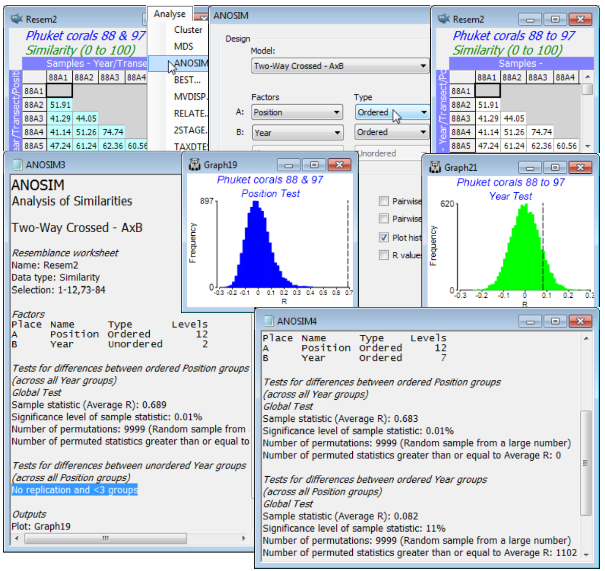
Run Analyse>ANOSIM>(Model•Two-Way Crossed - AxB)>(Factors A: Position Ordered & B: Year Unordered) on same resemblance selection as above, of the two years 88 and 97, together. This will, of course, produce a massively significant Position effect, with average R$^\text{O}$ = 0.69, and with (Max permutations: 9999) this is still off the top of the null distribution, p<0.01% (or, as a probability, P<0.0001). It is naturally a very powerful test, with $6 \times 10^{16}$ possible permutations.
It did not matter in this case whether the Year factor was defined as Unordered or Ordered, since there were only two years. The test for Year, removing the effect of Position by comparing years only within each of the 12 levels for Position, is doomed to failure, unsurprisingly. There are no replicates on which to base such a test (applying the above formula for an ordered test, a=2 so a!/2 = 1 and, whilst b=12 is large, powering up 1 still gives 1, i.e. there is only one permutation which is the observed configuration of the labels!). ANOSIM simply says No replication and <3 groups.
However, if we were to take off the selection, so reintroduce the full set of 7 years, and specify that both factors are ordered then there are ample steps in both the spatial gradient of 12 points and a temporal time trend of 7 points for an ordered test of either factor, removing the effect of the other. The Position test now gives a very similar R$^\text{O}$ = 0.69 as found for the two years alone but the Year test returns R$^\text{O}$ = 0.08, with about 1100 of the 9999 permutations created under the null hypothesis giving larger R$^\text{O}$ values than this (p<11%), a non-significant result. (Incidentally, note it is always true that a test of factor A is completely unchanged by whether factor B is assumed ordered or not).
In fact, whilst the original study postulated serial change in coral communities along the onshore-offshore transect, so that an ordered test for the Position factor seems very appropriate, it is not so clear that it is relevant to test for a monotonic inter-annual trend – a drift of the community in time, ever further away from its original configuration. Local impacts in some years may be dominant, and the possibility that these have a differential effect on the transect gradient (an interaction of a type) suggests a very different approach, using the Analyse>2STAGE routine, which we shall return to for these data in Section 14. Within the ANOSIM routines however, the 2-way crossed layout for an unordered factor with no replication leaves few options for a non-parametric test, though sometimes helpful is a fall-back test (available in PRIMER since the early versions), which is next described for the Exe estuary nematode data. Save and close workspace Phuket ws.
ANOSIM for 2-way crossed design with no replication (Exe study)
The 2-way crossed ANOSIM for an unordered factor, and with each combination of the two factors only having a single replicate, is covered in CiMC, Figs. 6.9 to 6.12, firstly for a treatment $\times$ block design and then for the example considered here of sites crossed with times. This is the inter-tidal Exe estuary nematode study, first seen at the start of Section 6 and used to demonstrate clustering and MDS, but here you should open the full data in a new workspace, i.e. the bi-monthly samples from the 19 sites, Exe nematodes bi-monthly in directory C:\Examples v7\Exe nematodes. It is the 6 seasonal samples, covering one year, which were averaged for each of the 19 sites in the earlier analysis of Exe nematode abundance. That there are clear site differences was obvious from the stark clustering of that data into 4 to 5 groups, but it is less clear whether there are site differences in the largest cluster, sites 12-19. So, as before, pre-treat the full data Exe nematodes bi-monthly with a 4th-root transformation and apply Bray-Curtis similarities, then select sites 12-19 (of course it does not matter whether you make the selection of these sites before or after calculating the transformations and similarities). The factors site and time are crossed because the same set of sites is returned to at each time. It is of interest here to test both, separately: are there differences among sites, removing the effect of times, and is there a seasonal effect, removing any site differences?
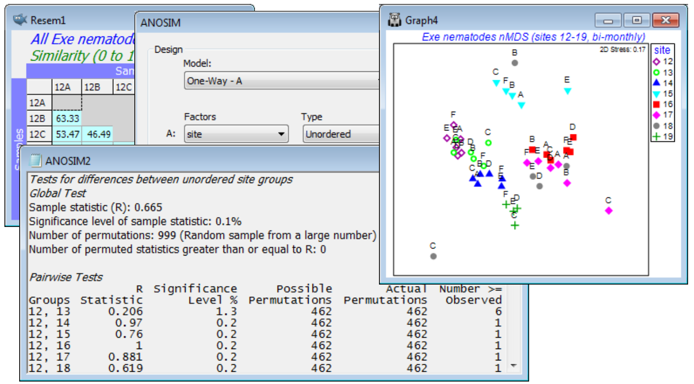
Analyse>ANOSIM>(Model:Two-Way Crossed - AxB)>(Factors A:site & B:time) both Unordered runs a different style of permutation procedure, testing for a site effect by asking whether there is evidence for commonality of the among-site pattern across the different times. For example, if the MDS plots of sites, displayed separately for each time (Fig. 6.12 in CiMC) show the sites grouping in the same way, that must imply there are site differences. To put it the other way round, under the null hypothesis that there are no site differences, the separate MDS plots for each time will have no common pattern and look like random rearrangements of each other. In fact the test operates, as with other ANOSIM tests, on the underlying resemblance matrix (ranks) rather than the MDS plots, and calculates an average of all pairwise correlations ($\rho_\text{av}$) between the among-site resemblance matrices for each time; $\rho_\text{av}$ will be near zero if there are no site effects. (The idea of this correlation $\rho$ between two triangular matrices, a type of non-parametric Mantel statistic, is at the core of most of Sections 13 & 14, and is discussed extensively in Chapters 6, 11, 15 & 16 of CiMC). ANOSIM then recomputes this $\rho_\text{av}$ statistic for random permutations of the site labels at each time (since for the null hypothesis there are no site differences), to obtain a null permutation distribution for $\rho_\text{av}$, and thus a significance test. CiMC, equations (11.3) to (11.4), gives details of the choices offered by the ANOSIM dialog, of rank correlation coefficient $\rho$ to calculate between pairs of resemblance matrices – Spearman rank is the best known and the default. Note that the routine automatically copes with a small number of missing samples (here caused by weather and/or tidal states at one or two sites on one or two occasions) because for each pair of times it can drop the sites which are not found in both configurations (called pairwise deletion of missing values), without having to drop those sites from the whole matrix (called listwise deletion). A satisfactory test does, however, need a decent number of shared sites available for all pairs of times (and for the test to have any power at all, some interactions must be small, otherwise no commonality is detectable – Chapter 6, CiMC).
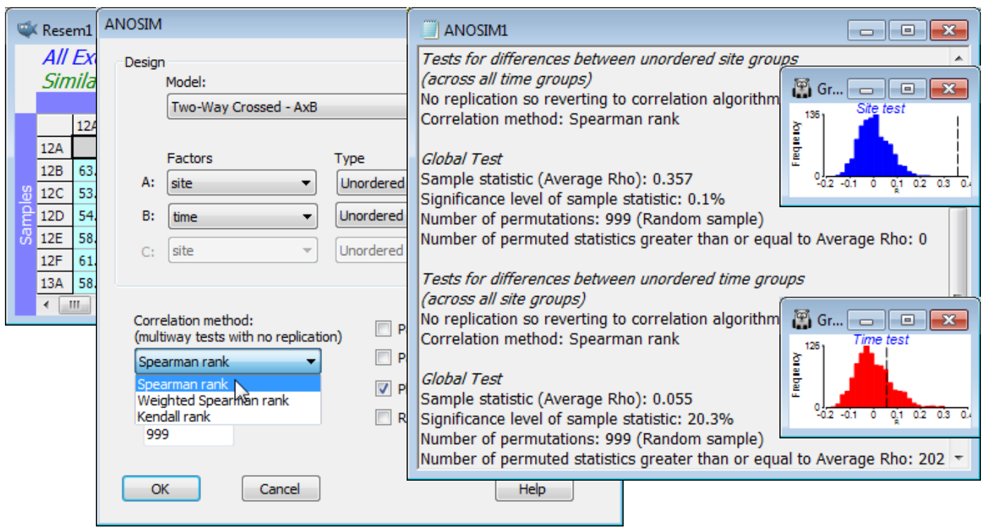
The results show a significant site effect ($\rho_\text{av}$ = 0.36, p<0.1%) but not evidence for a seasonal effect ($\rho_\text{av}$ = 0.06, p$\approx$20%, i.e. the relationships amongst times do not show commonality over all sites, or over sufficiently many of them to depart from random re-arrangement). The latter finding is not so surprising in a climatically mild region, given that generation times of meiofauna are measured in weeks. We might therefore be justified in strengthening the testing procedure for sites by running a 1-way ANOSIM on site, using the full set of 44 samples from sites 12-19, i.e. treating the different times as replicates. Now we can obtain tests between pairs of sites. Such pairwise comparisons are not available with the 2-way crossed analysis (without replicates) for obvious reasons – one cannot ask about commonality of pattern across 6 MDS plots, if each consists only of 2 sites, i.e. a single similarity value! From the 1-way ANOSIM results and the MDS of all samples, it is clear that most sites have significantly different and well-separated assemblages – with the exception of site 18, which is species-poor and has widely scattered replicates (time points) on the MDS, and site 12 vs 13 and site 16 vs 17, with low R values of 0.21 and 0.17 respectively. Close the workspace.
2-way nested ANOSIM (Calafuria macroalgae)
Subtidal rocky reefs, at ca 10m depth, at the Calafuria station in the Ligurian Sea, N Italy, were the subject of a clearance and recovery experiment by Airoldi L 2000 Mar Ecol Prog Ser 195: 81-92 (see also Clarke KR, Somerfield PJ, Airoldi L, Warwick RM 2006, J Exp Mar Biol Ecol 338: 179-192; both sources analyse a wider set of data than considered here). For 8 different times between October 1995 and September 1996 (factor A: named treatment, with levels 1 to 8), rock patches were cleared from three randomly chosen areas (factor B: area with levels 1 to 24, the three areas differing for each ‘treatment’, naturally). Three randomly chosen plots from each area (replicates) were then examined at the end of one year of recolonisation, and % area cover recorded of nine macroalgal taxonomic categories. The design is therefore a 2-way nested layout, with factor A (Trt) at the top level and B (Area) nested within A, denoted B(A) – replicates can be thought of as nested within B (replicates are always nested). Note that when defining the factor levels, PRIMER does not mind if you code the area levels as 1 to 24, or 1 to 3 repeatedly for each of the 8 treatments. If you use the latter, when 2-way nested is selected under Analyse>ANOSIM, and area is specified as nested, the routine will know that there is nothing in common between area 1, treatment 1 and area 1, treatment 2. But it may help you to code the area levels as 1 to 24, because the fact that area is nested, not crossed, with treatment will then be clear.
Open Calafuria algal cover from C:\Examples v7\Calafuria algae, and examine its factors with Edit>Factors. A strong transform is necessary to prevent the taxon category Algal turf from completely dominating, so transform with fourth root and calculate Bray-Curtis similarities between samples. The primary interest is in whether there are differences in recolonised macroalgal communities a year after clearance, depending on the time of year at which the clearance took place, i.e. a test of the treatment factor. But it is important to choose the correct replication level for this test. This is usually (some would argue, always) the level of variability immediately below treatment in the hierarchy, namely the areas not the plots, which are a level further down. So, one possibility is simply to average the three plots within each area and carry out one-way ANOSIM on the Trt factor (with 3 replicate areas per treatment). But what if there is absolutely no area effect, i.e. plots in different areas are no more dissimilar from each other than plots in the same area? Then it would seem reasonable to take plots as the replication level for testing treatment effects, and the much greater number of replicates will improve the sensitivity of that test.
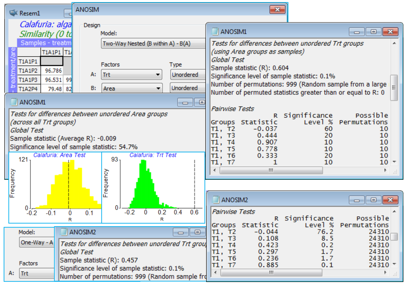
On the resemblances, take Analyse>ANOSIM>(Model: Two-Way Nested (B within A) - B(A))> (Factors A: Trt) & (B: Area), both of which are Unordered (the areas are randomly chosen from the region at each starting time, Trt, and though these starting times run sequentially through a year, a serial pattern for the algal recovery state a year later would not be expected – if anything it will be cyclic with the seasonality, see Section 14 for such tests). The routine then carries out two tests. Firstly, it tests the null hypothesis that there is no area effect. Nothing is assumed about treatment effects; these may or may not be present but need to be removed, in exactly the same way as for the 2-way crossed ANOSIM (i.e. R values contrasting among- and within-area rank dissimilarities are calculated separately for each treatment and averaged; permutations are constrained to shuffle labels among plots only over areas within a treatment, not across treatments, etc.). Secondly, the routine then always presumes that an area effect is present, so tests the treatments by averaging the plots within areas, thus using areas as the replication level for this test, by a 1-way ANOSIM. (In fact, the averaging is done on the rank dissimilarity matrix, which is then re-ranked for the 1-way ANOSIM – see CiMC). If there is demonstrably no area effect at all, so the test can use all 9 plots as replicates of a treatment, this needs a separate run of 1-way ANOSIM, ignoring the area factor.
The 2-way nested test for areas here gives average R = –0.01 (p$\approx$56%) and this near-zero R implies absolutely no suggestion of an area effect, making the 2-way test for treatments (averaging up to area level) unnecessarily conservative. It still gives a strongly significant global R of 0.60 but the conservatism is seen in the pairwise table, where comparisons are based on only 10 permutations (3 areas for each treatment). If, as is justified here, we ignore the area effect, the 1-way ANOSIM (9 plots per treatment) gives a pairwise table with 24,310 permutations for each comparison and thus clear inferences, e.g. T7 and T8 differ the most strongly from other times, with most R values in excess of 0.8, whereas pairs not involving these two times generally give R<0.4. If the initial test for area had given R>0 however, and certainly if it had been significantly so, on what will usually be a powerful test (many permutations), then it would not be justifiable to ignore the area effect and use plots as replicates: this would be non-conservative (pseudo-replication). Close the workspace.
3-way crossed ANOSIM (King Wrasse diets)
A dietary study of W Australian fish concerns composition by the volume of taxa (21 broad dietary categories: gastropods, bivalves, annelids, etc.) in the foregut of King Wrasse from one of 4 length-classes, caught in 3 locations in 2 periods of the year and 2 replicate times of sampling within each period (each replicate is a similar-sized pool of gut content of fish in each length-class). The data is Wrasse gut composition in C:\Examples v7\Wrasse diets. More detail is given in Chapter 6, CiMC; the analysis is from a wider study by Lek E et al 2011, J Fish Biol 78: 1913-1943.
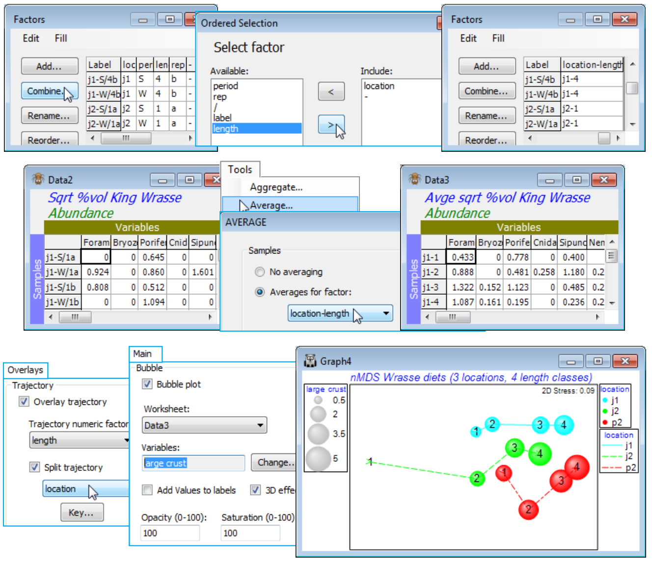
This is an example of a 3-way fully crossed design with replication, A$\times$B$\times$C, with A: location, B: length and C: period. A test of the null hypothesis of no effect, of each of the factors in turn, simply uses the earlier 2-way crossed design, e.g. with first factor A and second the flattened B$\times$C factor. The latter places all combinations of the levels of B and C in a single factor (using Edit>Factors>Combine and placing the B and C factor names in the Include box). The 2-way test for factor A now therefore constructs a 1-way ANOSIM R statistic for each combination of levels of B and C, and averages those, testing this against permutations constrained to stay within the B$\times$C levels. The same procedure is followed for each factor, so B is tested having removed the effect of A$\times$C, and C is tested have removed any effect of both A and B (or their interaction). So, whilst this could all be carried out by three separate runs of 2-way crossed ANOSIM, it is more conveniently (in PRIMER 7) performed by specifying the 3-way crossed design A$\times$B$\times$C. The resulting three average R values can then validly be compared, to determine the relative overall magnitude of the three effects.
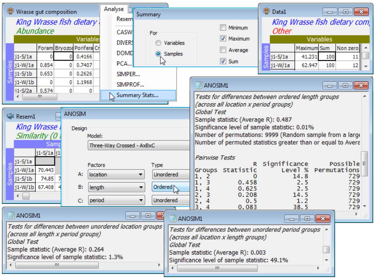
Here, the 3 levels of the location factor are not ordered, and there are only 2 periods (so whether treated as ordered or not is immaterial), but the 4 length classes of the predator wrasse are clearly ordered – the expectation is that, if the diet changes at all, it will do so in progressive fashion as the fish matures. So, check that the samples are already standardised to add to 100% across the dietary categories by Analyse>Summary Stats>(For•Samples) & (✓Sum) – you may want to leave other boxes checked also – and square-root transform then compute Bray-Curtis similarities, and input to Analyse>ANOSIM>(Model: Three-Way Crossed - AxBxC)>(Factors A: location) & (B: length) & (C: period), with B Ordered, specifying (Max permutations: 9999). The average R values show that B (0.49, p<0.01%) is the largest effect, then A (0.26, p<1.5%), but that C has no effect at all (0.00). The pairwise average R values for the length-class effect show the increasing differences in diet with difference in fish lengths, exactly as would be expected for an ordered factor (you may wish to re-run the analysis for an unordered B factor and note how this reduces its global average R value).
Given the clear absence of a period effect, a useful summary would be to average the (transformed) data over both the replicates and the periods (by Tools>Average and supply the combined factor for A$\times$B), recalculate the similarities and enter nMDS. The plot exemplifies a split trajectory, with Special>Overlays for length, splitting by location; you might also like to recreate the bubble plot of Fig. 6.15 of CiMC by adding a dietary component. Save and close the workspace (Wrasse ws).
3-way fully nested design (NZ holdfast fauna)
The 3-way fully nested design has factor C at the lowest level, nested in B at the mid level, which itself is nested in A at the top level, denoted C(B(A)). Factors can again be ordered or not, and the routine is essentially a repeated application of the 2-way nested design above – the first test, for C, is carried out simultaneously within the strata of all B levels (for every A level), the replicates in C levels are then averaged (in the same way as for the 2-way test, by averaging appropriate similarity ranks) and the test for B and A are now exactly that of the 2-way nested B(A) design. If replicates at the C level are not felt to be particularly reliable as snapshots of the community (each is species-poor, though pooled they give a fair representation of species presences at each level of C), it may be more efficient for the tests of B and A to pool or average the replicates in the data matrix, rather than the (rank) similarities, and run a 2-way nested B(A) ANOSIM with C levels as replicates.
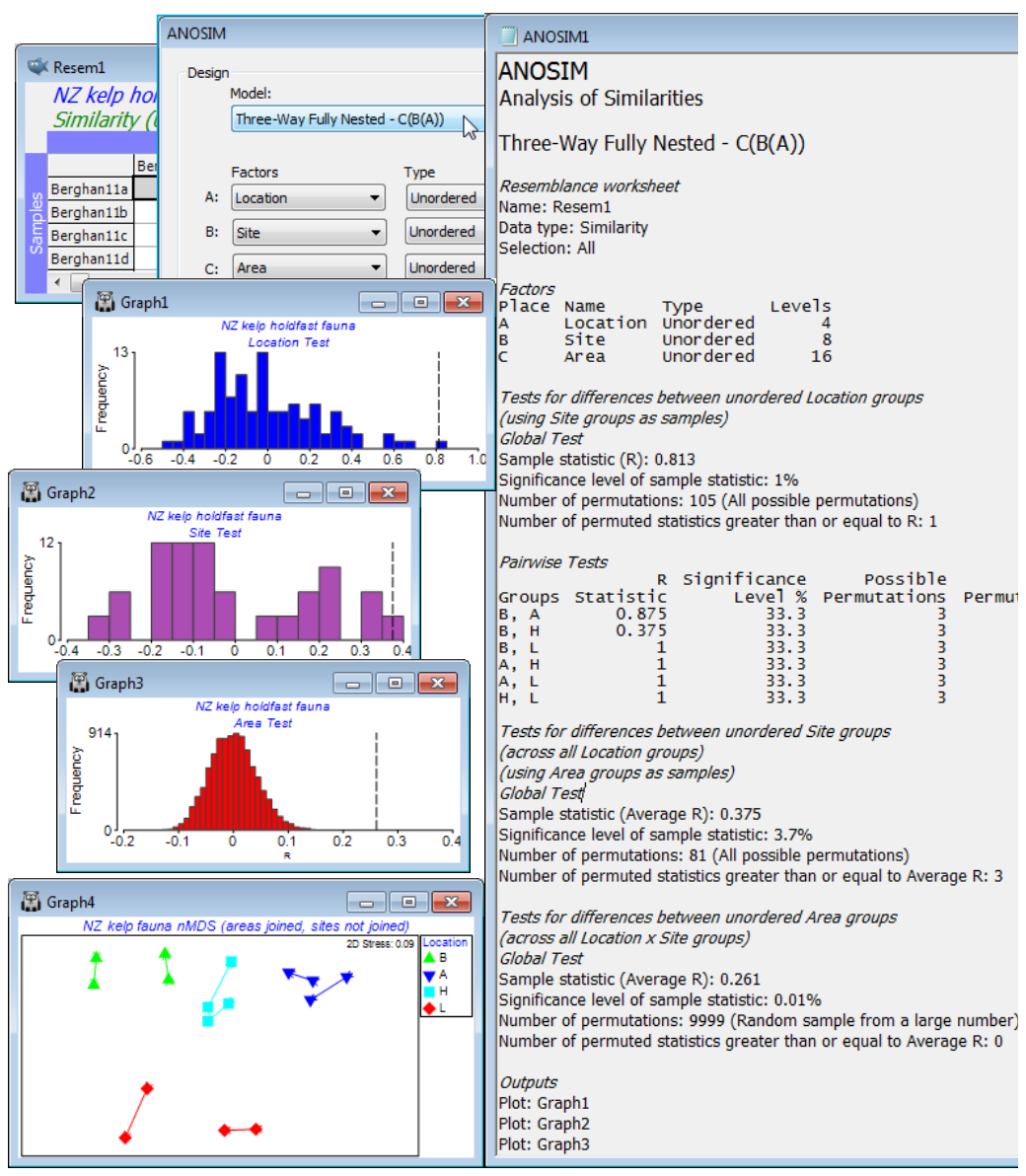
An example can be drawn from a data set of Marti Anderson and colleagues (Anderson et al 2005, J Exp Mar Biol Ecol 320: 33-56) distributed with the PERMANOVA+ add-on software, analysed in detail in the PERMANOVA+ manual (Anderson et al 2008) but which is also now to be found in C:\Examples v7\NZ holdfast fauna, as data file NZ holdfast fauna abundance. Chapter 6, CiMC gives the three-way nested ANOSIM tests for these data, see Figs 6.16 & 6.17. The macrofauna found in kelp holdfasts was sampled at 4 northern New Zealand Locations (A), with 2 Sites (B) per location, sampling 2 Areas (C) at each site, with 5 replicate holdfasts at each area. Clearly, Areas are nested in Sites, which are nested in Locations, C(B(A)). With only 2 sites per location and 2 areas per site, neither factor can be considered ordered, and there is also no case for considering the top-level locations ordered.
After square-root transformation and with Bray-Curtis similarities, Analyse>ANOSIM>(Model: Three-Way Fully Nested - C(B(A)))>(Factors A: Location) & (B: Site) & (C: Area), all Unordered, and (Max permutations: 9999). The resulting test statistics: R = 0.81 (p$\approx$1%) for the location test, and average R = 0.38 (p$\approx$1%) for sites and 0.26 for areas (p<0.01%), are again directly comparable with each other as measures of the extent to which stepping up the spatial level (replicates to areas, areas to sites, sites to locations) results in additional community differences – the largest effects are clearly at the location level. (Note the importance of interpreting the R values not the p values – the latter are always hijacked by the differences in number of permutations, here respectively 105, 81 and infinite, effectively, so that the smallest R value is actually the most significant!). Now produce a summary of these community differences at the different levels of the design, by averaging the square-rooted abundances over the replicate level (since the areas have all, sensibly, been given a different number, irrespective of the site or location, Tools>Average for factor Area will achieve this), then recalculating similarities and running nMDS. By careful use of symbol key changes, the means plot of Fig. 6.17, CiMC can be produced: plot symbols by Location; overlay trajectories by Area, split by Site; match up the line colours in pairs with those of the Locations and make all the lines continuous by clicking on the Site line key next to the plot; finally remove the Site line key by unchecking the (✓Plot key) box for Site on the Key tab, accessed through (say) General – easy!
3-way crossed /nested design (Tees Bay macrofauna)
The two other possible 3-way designs can be written C(A$\times$B) and B$\times$C(A). The first is straight-forward: an example might be of locations (A) each containing the same set of habitat types (B), and within each combination of habitat and location a number of sites (C) are randomly chosen, with replicates taken at each site. The ANOSIM tests are again effectively 2-way cases, with A and B flattened by combining them into a single factor (AB), so the design for testing C is the nested case C(AB), and the tests for A and B using the crossed 2-way A$\times$B design, with the levels of C as ‘replicates’ (averaging over the original replicates is, as usual, on the rank similarities). The 3-way C(A$\times$B) choice handles all this automatically, naturally, and again factors can be ordered or not.
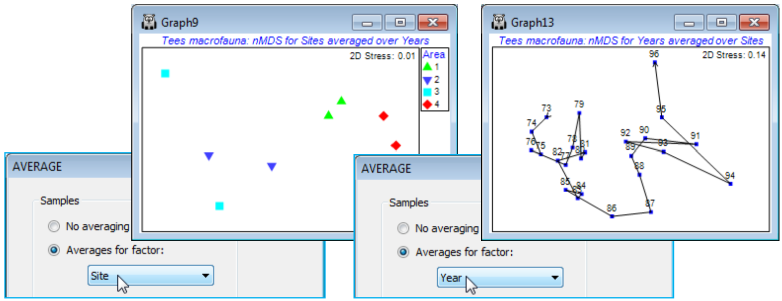
The remaining possibility B$\times$C(A), in which B is crossed with all levels of C, the latter nested in A, is more complex and for some tests requires variations of the 2-way test statistics (fundamentally still either average R, R$^\text{O}$ or $\rho$ constructions, however) and a modified permutation procedure in which whole sets of sample labels are permuted together. This is discussed extensively in CiMC, towards the end of Chapter 6 and in Table 6.4, and will not therefore all be repeated here. We will just use the same example as in CiMC to illustrate setting up and interpreting these tests. This is the Tees Bay macrofauna data introduced in Section 8 as an example of time-series trajectories in ordinations (see also Fig. 6.17 in CiMC), with workspace Tees ws and data Tees macrobenthic abundance in C:\Examples v7\Tees macrobenthos. Factors are Area (A), Year (B) and Site (C), with the 4 areas of Tees Bay (1-4) each containing two sites (a, b), each of which was resampled every September over the period 1973-96. Clearly the Sites are nested in Areas but Sites and Years are crossed (all sites sampled in all years), hence the design is B$\times$C(A). The data in this file has no replication at each site by time combination, the original multiple grab samples collected from a single sampling visit being regarded (perhaps a little harshly!) as pseudo-replication in time, and possibly even space, for September sampling of this community in a particular site and year – and thus the sample identifications from the multiple grabs (raw data) were averaged.
Areas are along a NW-SE transect of the coast but cannot be considered Ordered, since the mouth of the Tees estuary intervenes – see map in Fig. 6.17 of CiMC. [In fact, if the tests are done under the assumption that the areas are ordered 1 to 4, there is a failure to detect an area effect at all. This is a good example of the dangers of specifying the alternative hypothesis too narrowly – there is no power to detect an effect which does not conform to that alternative. Here the central areas 2 & 3 are different than the surrounding areas 1 & 4, probably because they are influenced by the Tees estuary mouth in the mid-Bay region]. Years, however, could be considered Ordered because there is interest in whether the communities show a (climate-change driven?) yearly trend, but could be entered as Unordered instead, if a simple serial drift is considered too narrow an alternative.
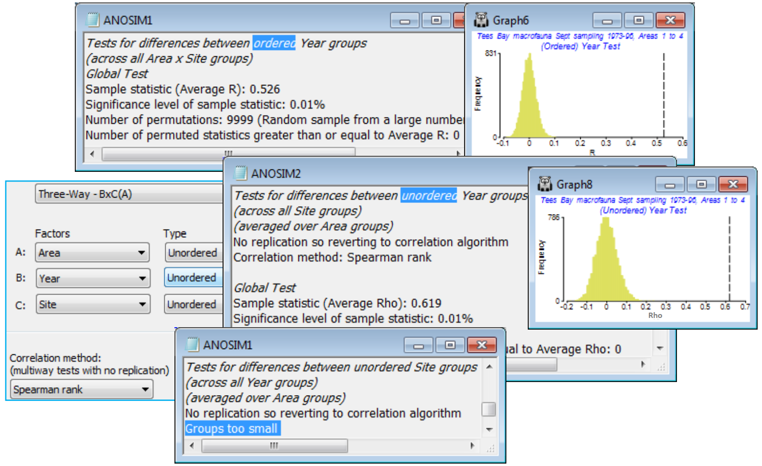
On 4th-root transformed data with Bray-Curtis similarities, Analyse>ANOSIM>(Model: Three-Way - BxC(A))>(Factors A: Area) & (B: Year) & (C: Site), with B Ordered, and then repeat the run with B Unordered, so the correlation method is needed: (Correlation method: Spearman rank).
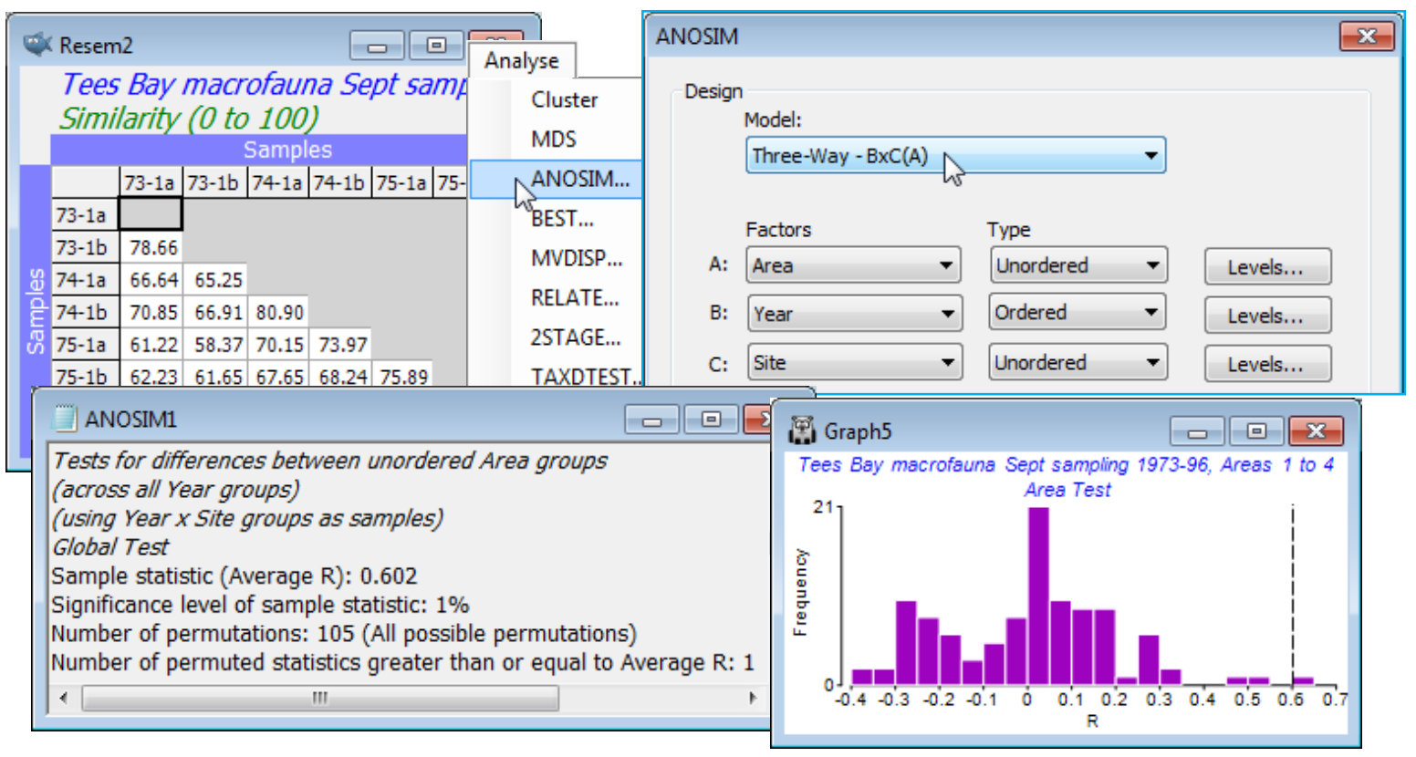
The (unordered) Area test has average R of 0.602 and this is the most extreme value in the 105 permutations (p<1%) – the permutation procedure here, a novel one for PRIMER, permutes the site labels within the areas but carries the full set of years with it, intact, reflecting the fact that the same sites are returned to each year, rather than randomly selecting two sites from each area at each time.
The ordered Year test gives an average R$^\text{O}$ of 0.526 which the null histogram shows to be as highly significant as we wish to make it. The unordered Year test needs to use a matching statistic ($\rho$) of the year pattern over sites or areas, as indirect evidence of a time effect from its spatial conformity. The average $\rho$ of 0.619 is also very highly significant. The $\rho$ value cannot be compared with the R$^\text{O}$ statistic, though both vary in the range (roughly) 0 to (definitely) 1, but the interpretation is clear – there is a broadly consistent time pattern across the region and it is fairly strongly serial.
A test of the third factor, Site, is clearly not possible. There are no replicates below this level to utilise, so ANOSIM tries instead the indirect route of matching the among-Site pattern over the set of Years – but with only two sites per area this must fail (giving a Groups too small statement in the results window). It has been important to retain Site as a factor however (rather than regarding it as a replicate) because the same sites are returned to each year and, with this 3-way procedure, the tests for Area and Year are designed to utilise that information in a more justifiable test.
The test results again justify a summary in terms of nMDS means plots. The area effect is clearly seen in an ordination using (transformed) data averaged over the years for each site, and the time series of years, now with (transformed) data averaged over all sites, certainly indicates a strong serial change (the same time series for the 4 area levels separately is seen in Fig. 6.17 of CiMC).