# 3-way fully nested design (NZ holdfast fauna)
The 3-way fully nested design has factor C at the lowest level, nested in B at the mid level, which itself is nested in A at the top level, denoted C(B(A)). Factors can again be ordered or not, and the routine is essentially a repeated application of the 2-way nested design above – the first test, for C, is carried out simultaneously within the strata of all B levels (for every A level), the replicates in C levels are then averaged (in the same way as for the 2-way test, by averaging appropriate similarity ranks) and the test for B and A are now exactly that of the 2-way nested B(A) design. If replicates at the C level are not felt to be particularly reliable as snapshots of the community (each is species-poor, though pooled they give a fair representation of species presences at each level of C), it may be more efficient for the tests of B and A to pool or average the replicates in the data matrix, rather than the (rank) similarities, and run a 2-way nested B(A) ANOSIM with C levels as replicates.
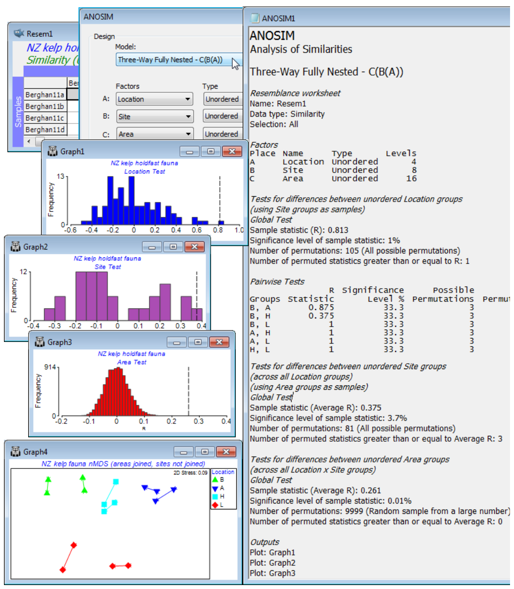
An example can be drawn from a data set of Marti Anderson and colleagues (Anderson *et al* 2005, *J Exp Mar Biol Ecol* 320: 33-56) distributed with the PERMANOVA+ add-on software, analysed in detail in the PERMANOVA+ manual (Anderson *et al* 2008) but which is also now to be found in C:\Examples v7\NZ holdfast fauna, as data file NZ holdfast fauna abundance. Chapter 6, CiMC gives the three-way nested ANOSIM tests for these data, see Figs 6.16 & 6.17. The macrofauna found in kelp holdfasts was sampled at 4 northern New Zealand *Locations* (A), with 2 *Sites* (B) per location, sampling 2 *Areas* (C) at each site, with 5 replicate holdfasts at each area. Clearly, *Areas* are nested in *Sites*, which are nested in *Locations*, C(B(A)). With only 2 sites per location and 2 areas per site, neither factor can be considered ordered, and there is also no case for considering the top-level locations ordered.
After square-root transformation and with Bray-Curtis similarities, **Analyse>ANOSIM**>(Model: Three-Way Fully Nested - C(B(A)))>(Factors A: Location) & (B: Site) & (C: Area), all Unordered, and (Max permutations: 9999). The resulting test statistics: R = 0.81 (p$\approx$1%) for the location test, and average R = 0.38 (p$\approx$1%) for sites and 0.26 for areas (p<0.01%), are again directly comparable with each other as measures of the extent to which stepping up the spatial level (replicates to areas, areas to sites, sites to locations) results in additional community differences – the largest effects are clearly at the location level. (Note the importance of interpreting the R values not the p values – the latter are always hijacked by the differences in number of permutations, here respectively 105, 81 and infinite, effectively, so that the smallest R value is actually the most significant!). Now produce a summary of these community differences at the different levels of the design, by averaging the square-rooted abundances over the replicate level (since the areas have all, sensibly, been given a different number, irrespective of the site or location, **Tools>Average** for factor Area will achieve this), then recalculating similarities and running *n*MDS. By careful use of symbol key changes, the means plot of Fig. 6.17, CiMC can be produced: plot symbols by Location; overlay trajectories by Area, split by Site; match up the line colours in pairs with those of the *Locations* and make all the lines continuous by clicking on the *Site* line key next to the plot; finally remove the *Site* line key by unchecking the (✓Plot key) box for Site on the **Key** tab, accessed through (say) **General** – easy!
[](https://learninghub.primer-e.com/uploads/images/gallery/2024-08/screenshotpage168a.png)