# Analysing between variables
The introduction above of the concept of ‘distances’ among species raises the issue of how best to compute *species similarities* – or more generally *variable associations* – taking the menu option of **Analyse>Resemblance**>(Analyse between•Variables). Several significant new developments in PRIMER 7 (see Section [10](https://learninghub.primer-e.com/books/primer-v7-user-manual-tutorial/chapter/10-wizards-and-species-analyses-basic-mva-coherence-plots-matrix-display-simper) and Chapter 7 of CiMC) on *shade plots* and *coherent species curves* concern better display and analysis techniques for characterising responses of individual (or groups of) species across the samples in space, time or over a changing environment. Two species are considered perfectly similar if they co-occur across samples – with numbers or biomass in strict proportion, for quantitative data. As with sample similarities, the issue of how to treat joint absence is often relevant here too – it would often be appropriate to regard the absence of two species at a particular site as uninformative (a clay-living and a gravel-living species are not similar because neither are found at sandy sites). A measure which captures this biological constraint well is the Whittaker Index of Association (IA), met earlier in this section. As remarked then, this will give the same outcome as standardising species (by total) and applying Bray-Curtis on the species. The (implicit) standardisation however will come unstuck with all-blank species, which must certainly be removed, and it is also almost always a good idea to remove all the ‘occasional’ species, rarely observed and with low abundances when they do occur. The various options for reducing to the ‘most important’ species were covered at the end of Section [3](https://learninghub.primer-e.com/books/primer-v7-user-manual-tutorial/chapter/3-highlighting-and-selection-select), and for standardising species near the start of Section [4](https://learninghub.primer-e.com/books/primer-v7-user-manual-tutorial/chapter/4-pre-treatment-options); these options would not usually apply when calculating sample similarities, but are important to eliminate wildly erratic, and not meaningful, similarities among rare species.
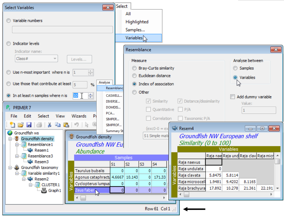
On the Groundfish density matrix, **Select>Variables**>(•In at least n samples where n is: 10). To see how many species are retained (61, in fact), click on the sheet’s final row which displays this in the status bar at the foot of the PRIMER desktop. Take **Analyse>Resemblance**>(Measure•Index of association) & (Analyse between•Variables) to create the species similarities (*Resem4* perhaps). Show that the same outcome is produced (*Resem5*) by putting the selected species from Groundfish density through **Pre-treatment>Standardise**>(Standardise•Variables) & (By•Total), followed by **Analyse>Resemblance**>(Measure•Bray-Curtis similarity) & (Analyse between•Variables).
[](https://learninghub.primer-e.com/uploads/images/gallery/2024-06/screenshotpage79.png)