# Basic MVA for environ-mental data
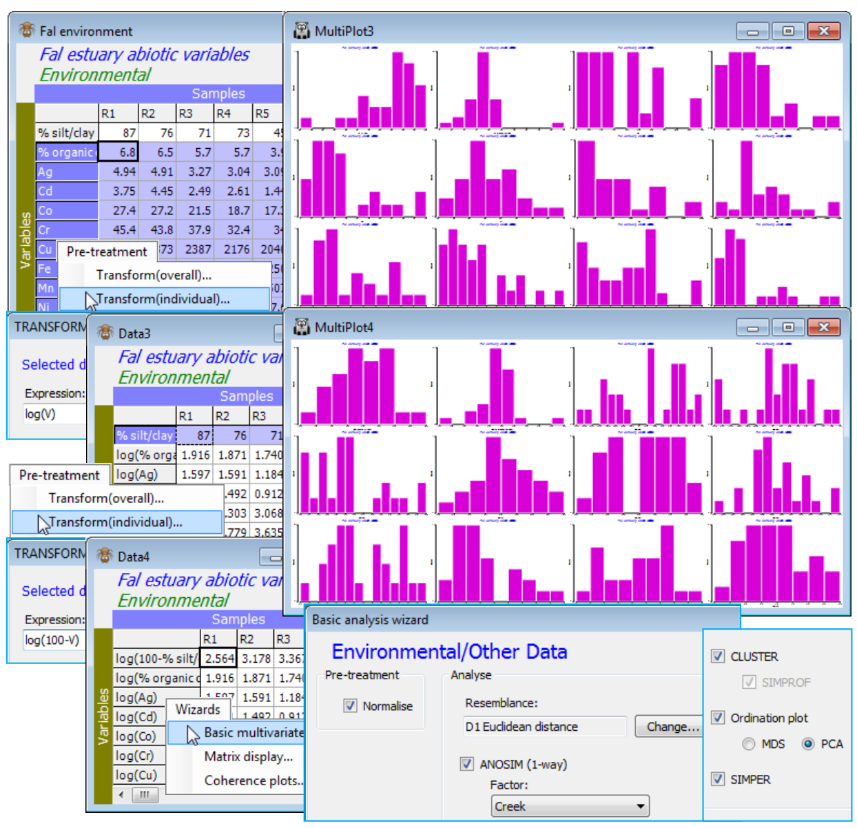
Finally, try running **Analyse>Basic multivariate analysis** on this environmental data matrix, Fal environment, to look at the pattern in the abiotic variables collectively, rather than singly (a match of this multivariate environmental structure to the multivariate assemblage pattern is the basis of the BEST routine, Section [13](https://learninghub.primer-e.com/books/primer-v7-user-manual-tutorial/chapter/13-linking-assemblage-to-environment-best-bio-env-linktree) & [14](https://learninghub.primer-e.com/books/primer-v7-user-manual-tutorial/chapter/14-further-matching-of-multivariate-patterns-relate-2stage-best-mvdisp)). The environmental analysis it provides is fairly skeletal – the dialog box only offers one pre-treatment option, (✓Normalise), which would usually be taken since abiotic variables are typically on non-comparable measurement scales. However, here, as is often the case, the concentration variables would benefit from a transformation before getting to this stage – their distributions are typically right-skewed, as can be seen from **Plots>Histogram Plot** or **Draftsman Plot**. It would be optimal therefore to highlight all except the *%silt/clay* variable and take **Pre-treatment>Transform (individual)**>(Expression: log(V)), see Section [4](https://learninghub.primer-e.com/books/primer-v7-user-manual-tutorial/chapter/4-pre-treatment-options), to give the new sheet Data3. The *%silt/clay* variable is of a very different type so it would not make sense to give it, automatically, the same transform as everything else. In fact, the histogram showed it to be left-skewed and Section [4](https://learninghub.primer-e.com/books/primer-v7-user-manual-tutorial/chapter/4-pre-treatment-options) then suggests a transformation expression such as *log(100-V)*, or *log(101-V)* if the maximum value of 100 is attained for one of the samples. So, on Data3, highlight this first row and **Pre-treatment>Transform (individual)**>(Expression: log(100-V)), giving Data4. A re-run of **Plots>Histogram Plot** shows a set of transformed variables which are much less prone to the effects of outliers on the upcoming ordinations and tests, being fairly symmetric over their ranges. \[If this pre-treatment stage seems all too much for you, at an early stage in your PRIMER experience(!), you could do worse than simply run **Tools>Rank variables** on Fal environment, which turns the 27 values for each variable into the ranks 1, 2, …, 27, and must totally remove the effects of any outliers, producing uniform distributions (at the price of loss of some sensitivity) – see under the Ranked variables heading in Section [11](https://learninghub.primer-e.com/books/primer-v7-user-manual-tutorial/chapter/11-general-data-manipulation-tools-further-pre-treatment) and an example of the resulting draftsman plot in Section [12](https://learninghub.primer-e.com/books/primer-v7-user-manual-tutorial/chapter/12-analysing-environmental-variables-draftsman-plot-pca). This would be one of the (rare) occasions when the on entry to the Basic MVA routine, you do not take the default (✓Normalise) option, since all ranks are on the same scale.\]
[](https://learninghub.primer-e.com/uploads/images/gallery/2024-08/screenshotpage174a.png)
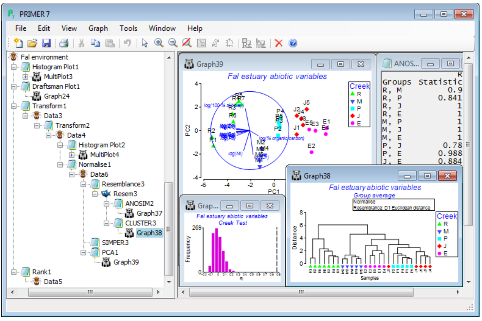
Now, on the final, selectively transformed data sheet, e.g. Data4, take **Analyse>Basic multivariate analysis**, and because PRIMER has been told that this sheet is of Data type•Environmental (see the window’s header line which will say *Environmental*, and if you need to change the type use **Edit> Properties**), the options offered by default will be (✓Normalise) & (Resemblance: D1 Euclidean distance), with the option to **Change** the latter to another resemblance measure. The analysis tools are now more or less the same as for biotic data, with (✓ANOSIM) proffered if a suitable factor exists (*Creek* in this case), and (✓Cluster), (✓Ordination plot) and (✓SIMPER). If ANOSIM is not checked, the default switches to (✓SIMPROF) tests on the standard clustering. The only difference now is that there is a choice of ordination options: (✓MDS) or (✓PCA), the former (again *n*MDS) being explicitly carried out using the supplied choice of distance coefficient, whilst PCA is only possible under an (implicit) Euclidean distance assumption. It follows that if a different distance measure has been selected, the PCA option is greyed out as unavailable. With ANOSIM run on the *Creek* factor and PCA for the ordination method, the Explorer tree under Fal environment is seen below. Note that PCA is run on the normalised data matrix, i.e. Data6 below, whereas for *n*MDS, the active sheet would have been the Euclidean distance matrix Resem3.
[](https://learninghub.primer-e.com/uploads/images/gallery/2024-08/screenshotpage175a.png)
It is again instructive to repeat the same steps as **Analyse>Basic multivariate analysis** manually. On Data4, take
**Pre-treatment>Normalise variables** (Section [4](https://learninghub.primer-e.com/books/primer-v7-user-manual-tutorial/chapter/4-pre-treatment-options)). The (✓Stats to worksheet) box is not ticked by default (if you check this, it just sends the mean and variance of each abiotic variable to a new sheet rather than listing them in the results window). On the normalised matrix, Data6, take **Analyse>Resemblance**>(Measure•Euclidean distance) & (Analyse between•Samples) to give Resem3, which is the active sheet for **Analyse>ANOSIM** and **Analyse>Cluster>CLUSTER**, both of which have exactly the same dialog as earlier, for analysing the biotic data in the *Creek* groups. As seen above, you may wish to add the *Creek* groups as symbols on the dendrogram with **Graph>Sample Labels & Symbols**. The other two routines start with the normalised data matrix Data6 as the active sheet. **Analyse>SIMPER** is set up as for the biotic data but with (Measure•Euclidean distance), which will be the default of course for data of environmental type. Finally, run Principal Components Analysis (Section [12](https://learninghub.primer-e.com/books/primer-v7-user-manual-tutorial/chapter/12-analysing-environmental-variables-draftsman-plot-pca)) on Data6, with **Analyse>PCA**>(Maximum no of PCs: 5) and the other defaults – there is rarely any need to interpret more than the first 5 PCs. A vector plot (in blue) will automatically be overlaid – see Section [8](https://learninghub.primer-e.com/books/primer-v7-user-manual-tutorial/chapter/8-multi-dimensional-scaling-non-metric-nmds-metric-mmds-combined-mds) for the various vector plots available – but this can obscure the plot and is turned off, and on again, on the **Graph>Special>Overlays** tab with the check box (Vectors✓Overlay vectors)>(•Base variables).
A run of Basic MVA with ANOSIM deselected again parallels the earlier options for biotic data.
The results show firstly that there are a lot of strong correlations among the abiotic variables, since the PCA results (PCA1) identify that the first 2 PCs account for 86.6% of the total variance and the first 3 PCs for 93.1% – these are very high figures. This is also seen in the eigenvectors, which give consistently large and negative values for all the metals (except *Cr* and *Ni*) on the PC1 axis, and negligible values on PC2. The vector plot shows these numbers graphically, with most metals thus increasing strongly towards Pill, Mylor and then, most strongly, the Restronguet creek samples (bubble plots would confirm this). In contrast, *%silt/clay*, *Cr*, *Ni* all have large eigenvectors on the PC2 axis, and relatively negligible ones on PC1, thus their vectors of increasing values point up or down the *y* axis (PC2) – *Cr* and *Ni* increase in the direction of the Mylor samples and Restronguet sites 1 and 2, as does *%silt/clay*. (Don’t forget here that the silt/clay variable used was reversed to *100-%silt/clay* before taking logs, so *%silt/clay* increases down the page). The *%organic carbon* variable has its really large value on PC3, and this will largely account for the rise from 87% to 93% of the explained variation. Its contribution to the full multivariate abiotic pattern is not seen therefore on this 2-d PCA, though a rotatable 3-d PCA plot is simply obtained by **Graph>Special**>(Plot type•3D) and shows that site J3 largely accounts for this third axis.
The PCA also demonstrates clearly how the different creeks separate out in terms of their environmental variables, and ANOSIM formally confirms this, with a very large overall ANOSIM R of 0.87, reflecting very large pairwise R values also. This is getting close to the point (R=1, Section [9](https://learninghub.primer-e.com/books/primer-v7-user-manual-tutorial/chapter/9-analysis-of-similarity-tests-unordered-and-ordered-anosim)) where all Euclidean distances among samples in different creeks are larger than any within a creek. The cluster analysis is also seen to divide up by creek, more or less perfectly (again, excepting J3). This abiotic analysis therefore gives the basis for a correlative interpretation (likely to be causal, though not necessarily) of the similar patterns from the earlier run of **Basic multivariate analysis** on the nematode assemblage data – see Section [13](https://learninghub.primer-e.com/books/primer-v7-user-manual-tutorial/chapter/13-linking-assemblage-to-environment-best-bio-env-linktree) for more on linking biotic and abiotic analyses.