# (Bristol Channel zooplankton)

Densities from 24 species of zooplankton at 57 sites in the Bristol Channel and Severn Estuary, collected by double-oblique net hauls, are in C:\Examples v7\BC zooplankton\\<ins>BC zooplankton density</ins>(.pri). The sampling sites were defined as a grid (Fig 3.2, CiMC), and samples taken through time over a single year and averaged to give one seasonally-averaged sample per site. There is thus no prior structure of groups and replicates within groups (though there is a natural salinity gradient, described by factor *Sal*, with 9 numeric levels). The original data is from Collins NR & Williams R 1982, *Mar Ecol Prog Ser* 9: 1-11, who identify four main clusters of sites. 

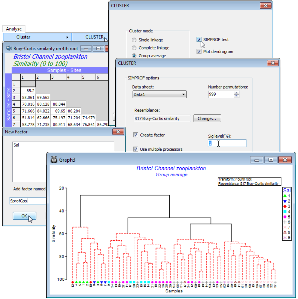
It is relevant to ask what the statistical evidence is for there being such a division at all, and if so, how much of the group structure can justifiably be interpreted. Open the data file <ins>BC zooplankton density</ins> and generate the cluster dendrogram from Bray-Curtis similarities on 4th root transformed densities (as in Sections [4](https://learninghub.primer-e.com/books/primer-v7-user-manual-tutorial/chapter/4-pre-treatment-options) & [5](https://learninghub.primer-e.com/books/primer-v7-user-manual-tutorial/chapter/5-resemblance-similarities-dissimilarities-and-distances)), then **Analyse>CLUSTER**>(Cluster mode•Group average), but this time taking the option (✓SIMPROF test). Look at the dialog under the **SIMPROF** tab, though the defaults probably be taken for (nearly) all: the matrix whose species rows will be independently permuted is <ins>Data1</ins>, the 4th root transformed data; no other choice than Resemblance: <ins>S17 Bray-Curtis similarity</ins> makes sense on the randomly permuted matrices since that was the choice on the real matrix; the % significance level is conventionally taken as <ins>5</ins> though could be more stringent, given ultimately that 7 tests are performed here, so change it to, say, <ins>1</ins>; the 999 permutations will typically be sufficient (for computing the mean, and a further 999 for departures $\pi$ from the mean) bearing in mind the computation needed to recompute and re-order the $n(n-1)/2$ similarities (with $n$ samples) for each permutation, and then repeat this through the dendrogram; and clearly the use of multi-cores in the processor is beneficial to that. The final group structure, from the series of SIMPROF tests, is placed in a factor, generating another dialog, (Add factor named: <ins>SprofGps</ins>).  

[![ScreenshotPage92a.png](https://learninghub.primer-e.com/uploads/images/gallery/2024-06/scaled-1680-/screenshotpage92a.png)](https://learninghub.primer-e.com/uploads/images/gallery/2024-06/screenshotpage92a.png)

With $n$ only 57 in this case, and with few tests needed, the SIMPROF procedure runs very quickly. The dendrogram shows the four groups of sites identified by Collins & Williams but now with firm statistical support: the black lines indicate groups that are established, with red lines showing a sub-structure from the clustering for which there is no statistical support from SIMPROF to permit interpretation. That the groups bear a strong relation to salinity is seen by displaying the salinity factor as a symbol, with **Graph>Sample Labels & Symbols**>Symbols:(✓Plot)>(✓By factor:<ins>Sal</ins>).