# BVStep from random starts
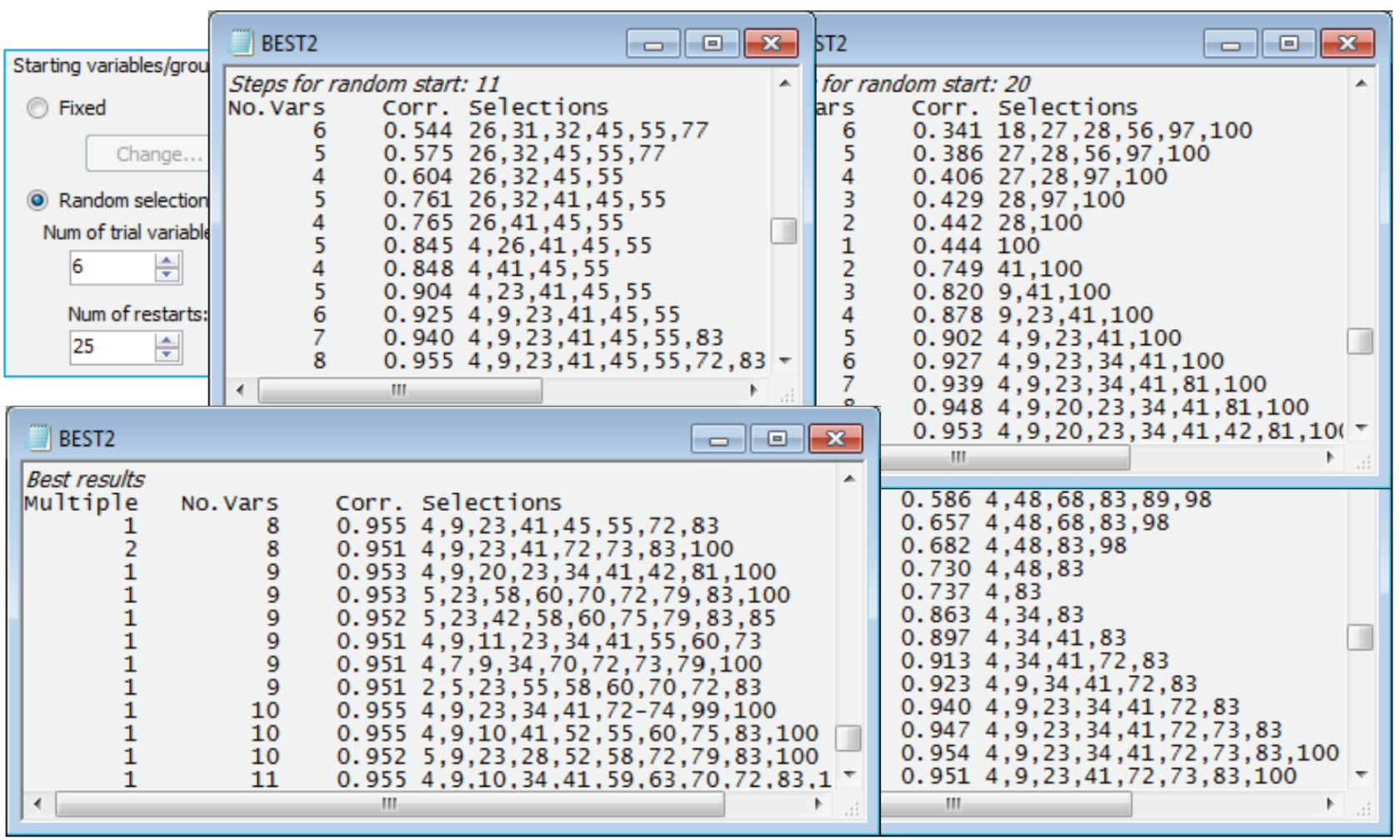
Starting the iterative search process from a blank species list is certainly not guaranteed to get you to the best solution (minimum number of species which give $\rho \ge$0.95) – it is easy to get trapped in a local optimum which is not the globally best solution (which can never be known for certain). In fact a marginally better solution, in the sense of involving only 8 species variables, can be found in this case. See this by re-running the routine from different starting places, having first reinstated the full 100-species transformed data matrix 4rt data by **Select>All** – this is important otherwise you will find yourself searching only through the 9 species! (You may also wish to remove highlights with **Edit>Clear Highlight**, though this is not important). The first dialog for **Analyse>BEST** (run on active sheet B-C on 4rt) is the same as previously, but on the BVSTEP dialog take (Starting variables/groups•Random selection)>(Num of trial variables/groups: 6) & (Num of restarts: 25). This starts the stepwise routine from a randomly chosen 6 species from the 100, and (Results detail: Detailed) and (Max num of best results: 25) on the last dialog will allow you to see the alternating backward elimination and forward stepping phases in the Results window. It also permits the final (*Best Results*) table to display all the solutions obtained – in best to worst order – in the event that they are all different (which they nearly all are in the case below!).
[](https://learninghub.primer-e.com/uploads/images/gallery/2024-10/screenshotpage262b.png)
Remember that these are not listed primarily in decreasing order of $\rho$ but in increasing order of the number of species. Only when two sets have the same number of species is the $\rho$ value (which has to be $\ge$0.95 for that solution to be listed at all) taken into account. You will obtain a different set than this (though probably overlapping), since a differing random number seed is used to select the starting species in every new run of the program. Occasionally, the search will end prematurely before 0.95 is reached, even though we know a value of 0.95 exists if we are searching the whole matrix (a value of 1 then exists!) – in that case try using Delta rho<: 0.0001, or even smaller, to try to keep the addition and deletion of species operating, and/or increase the number of restarts. The second-best solution above was found twice (see the *Multiple* column in the *Best Results* table) but many more than 25 restarts would probably be needed to be reasonably content that a 7-species solution could not be found. Setting out on an exhaustive search here rather misses the main point, though, that the impact and seasonal structure in the above MDS – which, importantly, is largely ‘signal’ because of the large sample sizes (we are not chasing ‘noise’) – can be displayed in just the same way by a small set of 8 or 9 species. A close look at the near-optimum solutions shows that many of the same species are involved in several of these.
In the further analysis in Fig. 16.3 of CiMC, from the Clarke and Warwick 1998 *Oecologia* 113 paper (and based on a somewhat larger number of species retained from the original *c*. 250), **BEST** is re-run, excluding this first subset of BEST-selected species, but again matching to the B-C on 4rt similarities from the retained set. In the above case, we therefore need to exclude species 4, 9, 23, 41, 45, 55, 72, 83 from the 4rt data matrix before entering it as the (secondary) worksheet to BEST. The quickest way of doing this, as seen earlier, is to copy and paste those 8 numbers to the **Select>Variables**>(•Variable numbers) box, then **Select>All** to leave them highlighted, and **Edit>Invert Highlighted** followed by **Select>Highlighted** will leave the remainder of the transformed 4rt data matrix selected for this second run of **BEST**. The matrix then needs to be **Tools>Duplicate**(d) in order to use the same trick to remove both the first and second species sets selected by BEST, if a third species set is sought. For the Morlaix data, about five entirely separate *species peels* can be found, all of which essentially reproduce the same multivariate pattern, indicating a high level of structural redundancy in the matrix.
This is the ‘opposite side of the coin’ from the *coherent curves* analysis we saw for this data in Section [10](https://learninghub.primer-e.com/books/primer-v7-user-manual-tutorial/chapter/10-wizards-and-species-analyses-basic-mva-coherence-plots-matrix-display-simper), where species were grouped into (about 8 or 9) distinct and characteristic sets in terms of their temporal patterns, seasonally and in response to the oil-spill and its aftermath. Each set contains several species which are able to substitute for each other, in the sense that their time patterns are statistically indistinguishable. Conceptually, it should be the combination of the (numerically more dominant) species drawn from each of these sets which tend to make up the above species peels, between them representing the range of temporal responses and therefore capable of recreating the community pattern for the full data set.
Close the Morlaix workspace – it will not be needed again.