# Environment bubble & vector plots

An important use for a bubble plot is in displaying the behaviour of a further measured variable, which has not been used in the multivariate analysis, across the sample positions on an ordination,  e.g. in superimposing environmental or contaminant variables one at a time, on a community MDS. Also, in this case, vector plots have a more useful role because there is a better chance of linearity, or at least monotonicity, of the relationships between abiotic gradients and community gradients –  also the rescaling of abiotic values implicit in a correlation coefficient is appropriate here, because environmental variables will usually be on different measurement scales. 

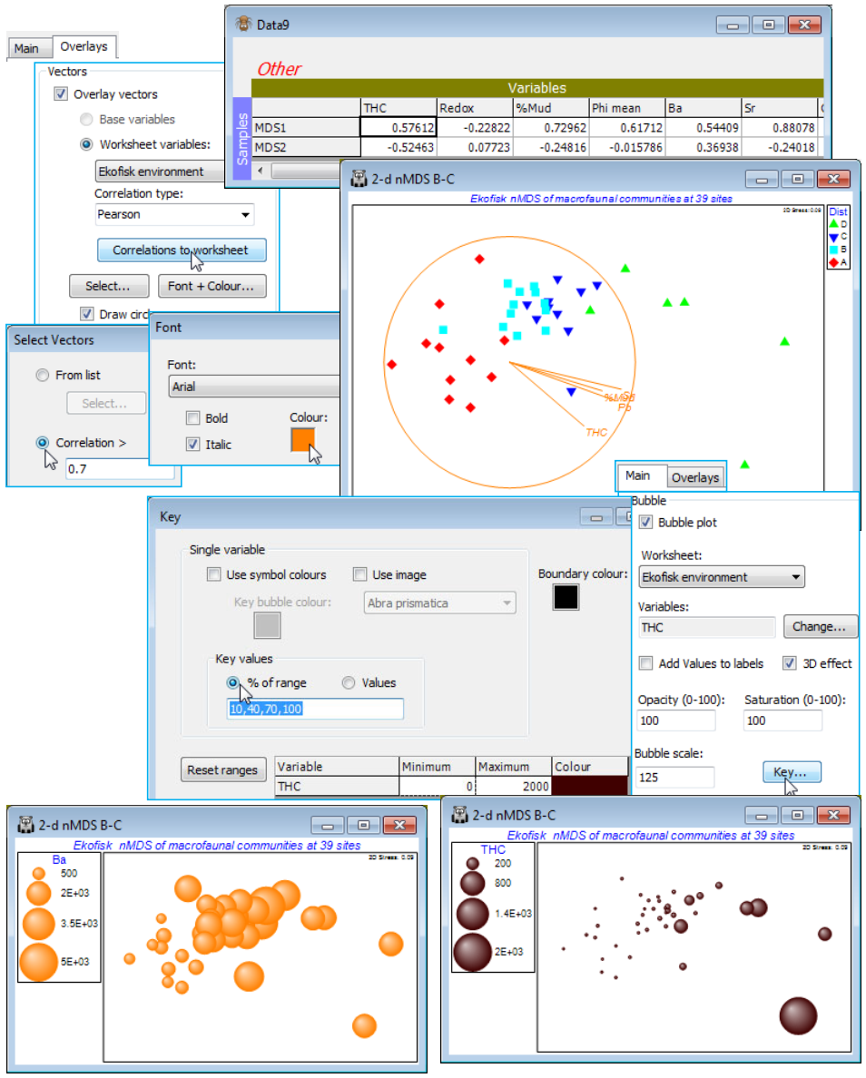
As an example, **File>Open** the <ins>Ekofisk environment</ins> sheet into the current workspace (if it is not already there from the transformation examples of Section [4](https://learninghub.primer-e.com/books/primer-v7-user-manual-tutorial/chapter/4-pre-treatment-options)). On the biotic <ins>2-d nMDS B-C</ins> plot, under **Special>Overlays**, retain (✓Overlay vectors) but change to (•Worksheet variables: <ins>Ekofisk environment</ins>) & **Select**>(•Correlation > <ins>0.7</ins>) to display only those abiotic variables with a high (multiple) correlation coefficient with the biotic ordination positions. The vector plot below shows these to be *THC*, *%Mud*, *Sr* and *Pb*. Those multiple correlations can be calculated by clicking the **Correlations to worksheet** button on the (✓Overlay vectors) dialog, which produces a worksheet of Pearson correlations of each abiotic variable with the ordination co-ordinates (MDS1, MDS2). These are the values obtained by projecting each vector onto the (*x*, *y*) ordination axes, which is how the vectors are constructed in this case. The length of the vector (the multiple correlation) is simply obtained by Pythagoras, e.g. for *THC*, $\sqrt{0.576^2 + (-0.525)^2} = 0.78$. \[For the technically minded, that this is equivalent to the multiple correlation coefficient from multiple linear regression of *THC* on the (MDS1, MDS2) co-ordinates follows from the fact that the MDS solution is rotated to PC’s, making the MDS axes uncorrelated\]. In addition, simple bubble plots (e.g. of *THC* and *Ba*) can be drawn as before, using **Main**>(✓Bubble plot>Worksheet: <ins>Ekofisk environment</ins>).

[![ScreenshotPage138a.png](https://learninghub.primer-e.com/uploads/images/gallery/2024-07/scaled-1680-/screenshotpage138a.png)](https://learninghub.primer-e.com/uploads/images/gallery/2024-07/screenshotpage138a.png)

The vector plot, though not as unsatisfactory as when superimposing species, can again be seen to miss an important relationship here by comparison with the bubble plots. The pattern of *Ba* is not a linear one and thus does not give a very strong correlation, but it is distinctive and instructive, since barite is a component of the drilling muds dispersing into the marine environment. The bubble plot shows that *Ba* values are consistently higher around the oilfield but drop to background levels at about 3-4km – another example of a threshold change not optimally captured by correlation. Note that plots here used untransformed abiotic variables, which is visually informative, but there is a good case for instead using the selectively transformed sheet (<ins>Data3</ins>) deemed appropriate for these variables in Section [4](https://learninghub.primer-e.com/books/primer-v7-user-manual-tutorial/chapter/4-pre-treatment-options); e.g. this would reduce the dominant effect of the large outlier in *THC*.