# (Fal estuary copepods)

Sediment copepod assemblages (and other fauna) from five creeks of the Fal estuary, SW England, were analysed by Somerfield PJ, Gee JM, Warwick RM 1994, *Mar Ecol Prog Ser* 105: 79-88.  The sediments of this estuary are characterised by high and varying concentrations of heavy metals, a result of tin and copper mining over hundreds of years. The copepod data consist of 23 species found in 27 samples, consisting of 5 replicate cores spanning each creek (Mylor: M1-M5; Pill: P1-P5; St Just: J1-J5; Percuil: E1-E5; and 7 from the largest creek, Restronguet: R1-R7). These are in directory C:\Examples v7\Fal benthic fauna, worksheet <ins>Fal copepod counts</ins>(.pri), with a factor *Creek* identifying samples from the 5 creeks. There are also environmental cores (of silt/clay ratios, heavy metals etc.) matching these 27 sample locations, held in an Excel file <ins>Fal environment</ins>(.xls), plus nematode densities, macrofaunal counts and biomass, and associated aggregation files. 

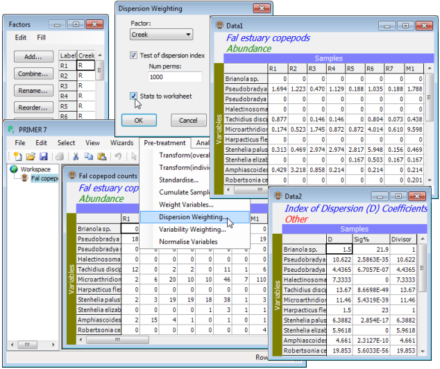
**File>Open** the copepod data and take **Pre-treatment>Dispersion weighting**>(Factor: <ins>Creek</ins>) & (✓Test of dispersion index) & (Num perms: <ins>1000</ins>) & (✓Stats to worksheet). The <ins>Data1</ins> sheet gives the dispersion weighted counts, which are either ready to go into the **Analyse>Resemblance** step of the next section, or could be mildly transformed before they do so, as shown earlier with **Pre-treatment>Transform(overall)**>(Transformation: <ins>Square root</ins>). There seems little need for the latter, however, since the dispersion weighting has already succeeded in downweighting the larger, erratic counts coming from *P. littoralis*, *R. celtica*, *E. gariene* and *T. discipes* and the somewhat less erratic *P. curticorne* and *M. falla* – the matrix <ins>Data1</ins> now has no dispersion-weighted ‘counts’ in double figures, and the subsequent untransformed analysis will not be dominated by a small set of species.  In three columns, <ins>Data2</ins> gives: the mean dispersion indices $\overline{D}$  for each species; the evidence for clumping (i.e. the % significance level  for a test of $\overline{D} = 1$); and the actual divisor used for that species row, which is 1 if the test does not reject this hypothesis at 5% (or better). Thus, *T. discipes* values are divided by 13.67 but *Brianola sp*. remains unchanged, though $\overline{D} = 1.5$. You might now like to run the routine again for the <ins>Fal nematode abundance</ins> file, which inspection shows must be numbers scaled up to a density, not real counts (e.g. there are no entries of 1!). The tick box for the test must be unchecked,  the resulting $\overline{D}$  values are all >>1, but weighting by $\overline{D}$  is still justifiable.

[![ScreenshotPage60a.png](https://learninghub.primer-e.com/uploads/images/gallery/2024-05/scaled-1680-/screenshotpage60a.png)](https://learninghub.primer-e.com/uploads/images/gallery/2024-05/screenshotpage60a.png)