# Higher-d & scree plots (WA fish diet)
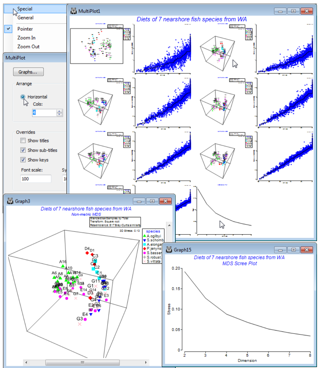
Run *n*MDS at a wider range of dimensionalities than the default and ask for a *scree plot*: **Analyse> MDS>Non-metric MDS (mMDS)**>(Min. dimension: 2) & (Max. dimension: 8) & (✓Scree plot), taking the other defaults (i.e. including Shepard plots). On the resulting multi-plot, Multiplot1, take **Graph>Special**>(Arrange•Horizontal)>(Cols:4) to make sure the MDS plots and their associated Shepard diagrams are arranged in two pairs across each of the 4 rows, finishing with the scree plot.
Clicking on the 2-d configuration you can see that though there are some clear differences in the dietary assemblages for some fish species, the stress of the plot is high (0.19), reflected in the large scatter in its Shepard diagram. The 3-d (& 4-d) solutions are noticeably better, with the stress falling to 0.13 (and then 0.09); the scree plot shows this initially quite steep decline (stress must always decline as the number of dimensions available, to display the relationships among samples, increases). Of course, solutions in higher than 3-d can only display three co-ordinates at a time, so the configurations in the multiplot all show only axes MDS1, MDS2, MDS3. Whilst sets including some higher axes could be viewed for the $\ge$4-d solutions, e.g. MDS1, MDS2, MDS4, the primary visualisation here should be the 3-d MDS, which has a stress at ‘acceptable’ levels (see discussion on stress levels in CiMC, Chapter 5). Click on the 3-d plot in the multiplot (Graph3) and **Zoom In**, remove the uninformative labels by unchecking (Labels✓Plot) from the **Samp. Labels & Symbols** tab, remove the history by unchecking (✓Plot history) on the **General** tab, edit the title and delete the subtitle by removing its content on the **Titles** tab. You may also want to change the colour or symbol for some of the species by clicking on the key, which sends you to the Key dialog box, as previously seen. Finally rotate the 3-d axes manually by **Graph>Rotate Axes** (or the [](https://learninghub.primer-e.com/uploads/images/gallery/2024-06/rotateicon.png) icon), to note how some fish species (e.g. *S. vittata*) feed widely across the dietary space and others are more specific (e.g. *S. robustus*). Testing of these dietary differences requires ANOSIM (Section [9](https://learninghub.primer-e.com/books/primer-v7-user-manual-tutorial/chapter/9-analysis-of-similarity-tests-unordered-and-ordered-anosim)).
[](https://learninghub.primer-e.com/uploads/images/gallery/2024-07/screenshotpage127a.png)