# (King Wrasse diets)

A Western Australian study of the dietary assemblages of a single fish species (King Wrasse) were analysed as a 3-way crossed ANOSIM design, followed by an *n*MDS means plot, in Section [9](https://learninghub.primer-e.com/books/primer-v7-user-manual-tutorial/chapter/9-analysis-of-similarity-tests-unordered-and-ordered-anosim). The three factors were samples taken at 3 *locations* (j1, j2, p2), at 2 *periods* in the year (S, W), and for wrasse of 4 *length*-class ranges (1-4), with 2 replicate (pools of) fish guts for each combination. Matrix entries were the percentage of the gut material by volume for each of 21 dietary categories, thus already sample-standardised, i.e. each sample adds to 100%. Square root transformation was taken prior to Bray-Curtis similarities, and the ANOSIM tests showed no effect of period at all (an average R value of 0.0), so the summary *n*MDS means plot averaged the (transformed) matrix over replicates and periods, to give 12 samples (3 locations by 4 length-classes). It is these averages that we will now input to Matrix display, to attempt to identify the dietary categories that it would be useful to display in a bubble plot on this averaged *n*MDS, which shows the rather weak location differences (average R = 0.26, p<1.5%) and stronger, <u>ordered</u> length-class effect (average R$^\text{O}$ of 0.49, p<0.01%). In fact, this was the analysis that suggested a bubble plot of the *large crust*(acean) category seen in Section [9](https://learninghub.primer-e.com/books/primer-v7-user-manual-tutorial/chapter/9-analysis-of-similarity-tests-unordered-and-ordered-anosim) – as noted earlier, other techniques for identifying contributing species, such as SIMPER (see end of this section), are not well suited to dissecting ordered changes. 

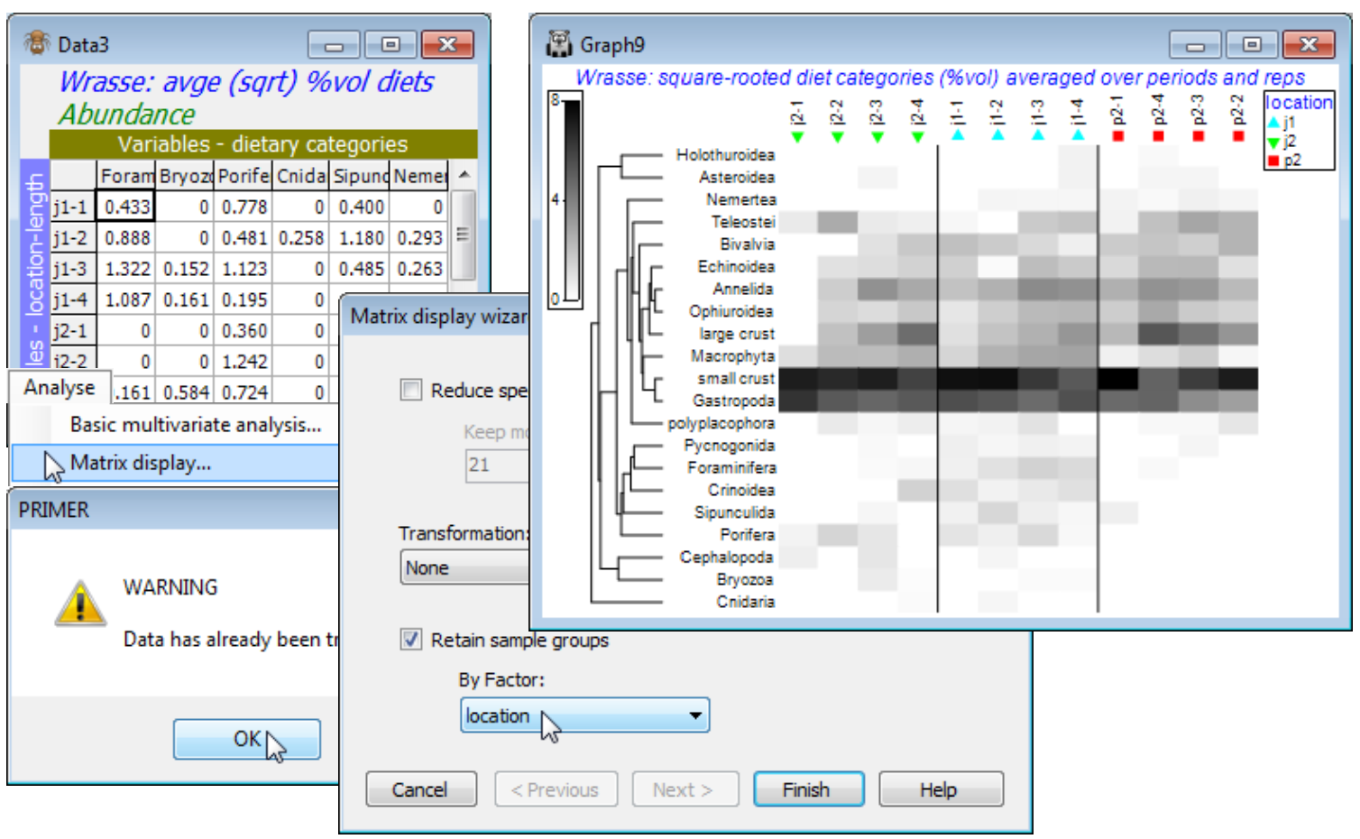
So, open <ins>Wrasse ws</ins>, or if unavailable, open <ins>Wrasse gut composition</ins> in C:\Examples v7\Wrasse diets and square-root transform this matrix. \[As an aside, from the **Edit>Factors** sheet you will see how a **Combine** of the factors: <ins>location</ins>, <ins>-</ins>, <ins>period</ins>, <ins>/</ins>, <ins>length</ins> and <ins>rep</ins> has produced a combined factor then **Renamed** <ins>label</ins>, which was highlighted and copied to the clipboard (Ctrl-C), then the factor sheet saved, **Edit>Labels>Samples** taken, the existing labels (which were previously just integers 1, 2, 3, …) highlighted, and the more meaningful labels pasted over them (Ctrl-V).\] We shall need a simpler **Combine** here under **Edit>Factors**, of <ins>location</ins>, <ins>-</ins> and <ins>length</ins>. Then run **Tools>Average**>(Averages for factor: <ins>location-length</ins>) on the root-<u>transformed</u> form of the matrix and enter this to **Wizards>Matrix display**. You will get the warning message: *Data has already been transformed* but this can safely be ignored for averaged data of this sort, where it makes good sense to do the transformation before the averaging (the issue of how best to create averages is briefly mentioned in Section [9](https://learninghub.primer-e.com/books/primer-v7-user-manual-tutorial/chapter/9-analysis-of-similarity-tests-unordered-and-ordered-anosim) and again at the start of Section [17](https://learninghub.primer-e.com/books/primer-v7-user-manual-tutorial/chapter/17-bootstrap-regions-for-group-means-bootstrap-averages), but options are discussed in more detail in CiMC). The warning message is here to guide users towards running **Matrix display** on the raw data, and taking any necessary transformation within the routine, since it is (arguably) the preferred option for the species similarities to be computed on untransformed data, but this is by no means a ‘hard and fast’ rule, and here it is natural to run Matrix display on the (transformed then) averaged matrix – and not to request a further transformation, of course. Take **OK** on the warning message, <u>un</u>check (✓Reduce species set) since there are only 21 ‘species’ (dietary categories), take (Transformation: <ins>None</ins>) and (✓Retain sample groups>By factor: <ins>location</ins>), to give the initial shade plot shown.
 
[![ScreenshotPage183a.png](https://learninghub.primer-e.com/uploads/images/gallery/2024-08/scaled-1680-/screenshotpage183a.png)](https://learninghub.primer-e.com/uploads/images/gallery/2024-08/screenshotpage183a.png)

Note that the submitted matrix had samples (location-length combinations) as rows, and variables (dietary categories) as columns, but the shade plot will always transpose the matrix in that case, to give a shade plot with ‘species’ as the *y* axis and samples on the *x* axis – there is no choice here. The resulting plot does still need some fine tuning, as usual, under three **Graph** dialogs (right-click over the plot). Firstly, **Samp. Labels & Symbols**>(Labels✓Plot)>(✓By factor <ins>length</ins>) would make the length categories more prominent. More importantly, these are seen not all to be in the correct sequence – their order was determined by the initial run of **Matrix display**, with its inbuilt attempt to diagonalise the shade plot (subject to the constraint of keeping location levels together). If we want to order by the *length* factor, it has to be numeric (we have seen this before with factors) and it is already numeric in this case – the size groups 1 to 4. So, on the **Special>Reorder** dialog, take Samples>(Order•Numeric factor)><ins>length</ins>, leaving all other conditions unchanged, except to change the number of restarts to 9999 – this runs very quickly with the small number of species.