# Metric MDS for ordinating few points
Though usually greatly inferior to *n*MDS for typical ordinations from community similarities (e.g. with coefficients from the Bray-Curtis family), purely metric MDS (*m*MDS) becomes a valuable tool for ordinations based on only a handful of samples, when the information content of the ranks in a similarity matrix is often insufficient to constrain the problem. E.g. for 4 samples we have only the 6 numbers, 1, 2, 3, 4, 5, 6(!), and an infinity of stress zero solutions may be possible in *n*MDS. *m*MDS uses the actual (dis)similarities as the distances between points and solves a perfectly well-defined problem – even as few as 4 points in 2-d is unlikely to have an exactly zero stress solution. Such small-scale ordinations usually arise as means plots: averages are carried out for a number of groups over replicates or other crossed factors (e.g. averaging over times for a number of sites, or *vice versa*). This is achieved by **Tools>Average** on the transformed data matrix and calculation of the resemblances among these averaged samples (or, in the context of PERMANOVA+, by taking the menu item **Distances among centroids** on the original resemblance matrix, see Anderson et al, 2008, the PERMANOVA+ User manual). It is precisely such situations, with very few samples and thus few points on the Shepard diagram, where linearity of the distance *vs* dissimilarity relationship may be viable. Furthermore, the likelihood of the straight line going through the origin is increased, i.e. two means from exactly the same community structure will tend to have very low dissimilarity, because sampling variability is reduced by the averaging over replicates or other factors.
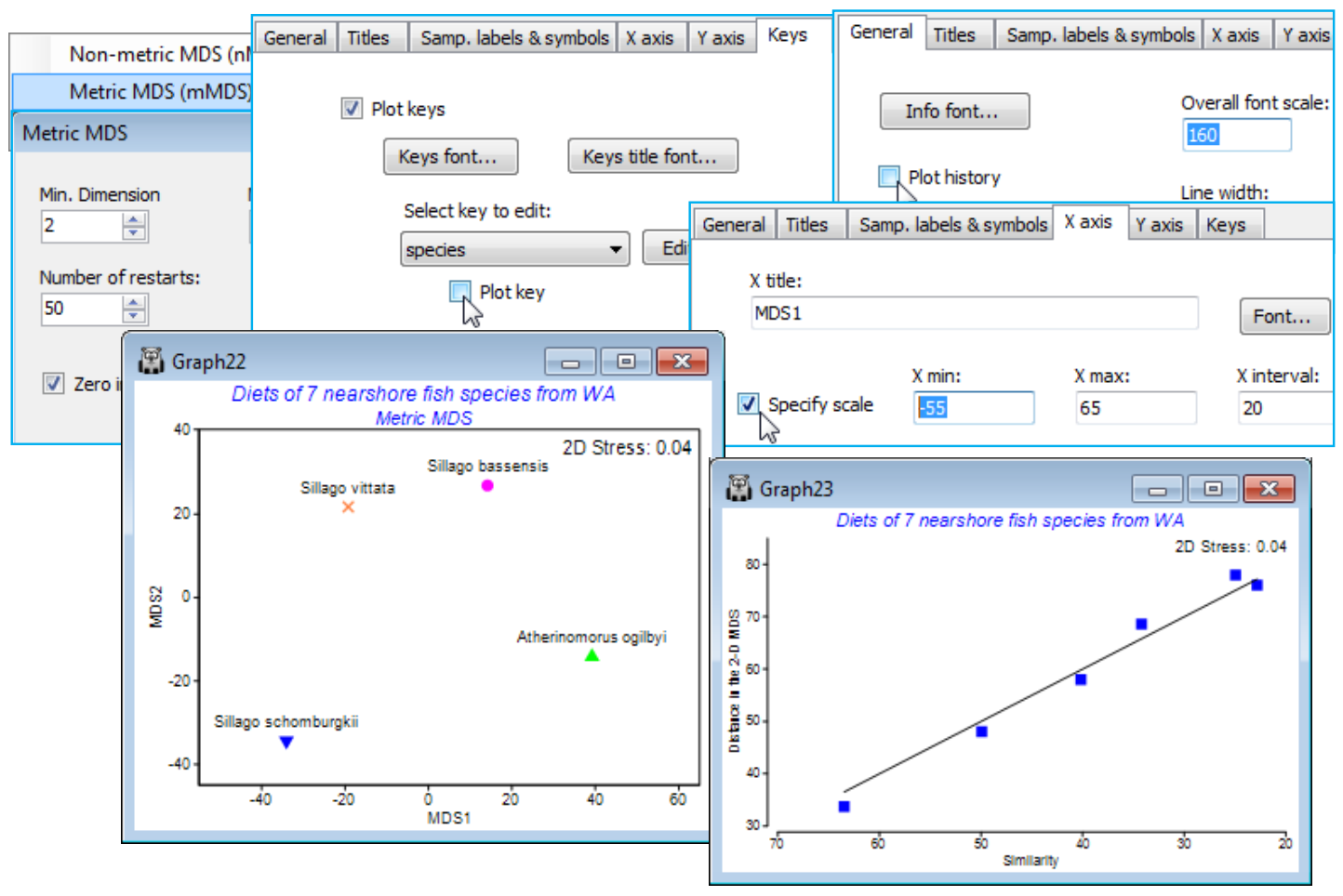
As an example, re-open the WA fish ws workspace of dietary assemblages of 7 species of Western Australian fish, for which averages over the (transformed) replicate gut samples from each species were calculated a few pages ago (in the presentation of segmented bubble plots). From the Bray-Curtis resemblance matrix computed on those averages, **Select>Samples**>(•Factor levels)>(Factor name: species)>**Levels** and Include only the four species with reasonably large numbers of samples – the three congeneric *Sillago* species (*S. schomb.*, *S. bassen.*, *S. vittata*) and *A. ogilbyi*, which all have between 10 and 16 replicate pools (each of 5 fish guts). Run **Metric MDS (mMDS)** on this 4 sample resemblance matrix. This only has 6 entries and *n*MDS would have insufficient information to be reliable (although not actually collapsing to a degenerate solution in this case, though it will often do so for 4-sample plots). *m*MDS, however, is seen to be valid – the 2-d Shepard diagram shows a reasonably convincing low-stress linear relationship, passing through the origin – and the 2-d ordination actually places these 4 points in very similar relationship to each other as seen in the previous *n*MDS plot for all 7 species (in that case, *n*MDS had plenty of information to work with, since there were 21 resemblances to rank). Note that the tidying up of this plot used: the **General** tab to uncheck (✓Plot history), increase (Overall font scale) and increase (Size) on **Info font** (stress value); **Samp. labels & symbols** to (Label✓By factor species full name) and to increase (Symbol> Size); both **X axis** and **Y axis** tabs to (✓Specify scale); and the **Keys** tab to uncheck (✓Plot key).
[](https://learninghub.primer-e.com/uploads/images/gallery/2024-07/screenshotpage148a.png)
Resave the workspace as WA fish ws for use in the next section, and close it.