# (Morlaix macrofauna, Amoco-Cadiz oil spill)
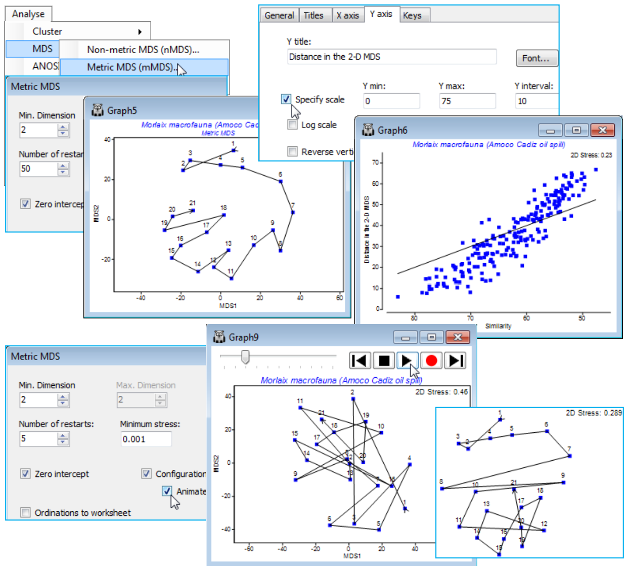
Close the World cities worksheet (it will not be needed again) and re-open workspace Morlaix ws, from earlier in this section. It contains the data sheet Morlaix macrofauna abundance, fourth-root transformed and with Bray-Curtis similarity matrix, Resem1, on which to carry out 2-d *m*MDS, with **Analyse>MDS>Metric MDS (mMDS)**, taking all the default options, and making the time factor the labels rather than the symbols, on **Samp. labels & symbols** – you should also join the points in *time* order as previously demonstrated, with **Special>Overlays**>Trajectory. The below also adjusts the scales of the Shepard plot by clicking on them (**X axis** & **Y axis** tabs). You might also enjoy repeating this 2-d MDS with, say, (Number of restarts: 5) & (Minimum stress: 0.001) and (✓Animate) switched on. Make sure that you make the above symbol and label changes, and especially the trajectory overlay, before starting the animation, with [](https://learninghub.primer-e.com/uploads/images/gallery/2024-07/playicon.png) . Even with the rather small number of points here (21) and the clear pattern, note how often the convergence does get trapped in a sub-optimal solution. This is also clear from the results window, mMDS1, from the initial run with 50 restarts, with only 20-30% of those converging to the (probably) lowest stress of 0.235.
Marginally higher stress is to be expected from an *m*MDS solution than an *n*MDS one, even if the Shepard diagram does show a linear fit through the origin to be an excellent description of the relationship of dissimilarities to plot distances – this is because *n*MDS’s monotonic regression can make fine-scale steps to ‘chase’ the data even when displaying essentially a straight line (especially if there are few samples and therefore not too many points on the Shepard plot to ‘chase’). But a high stress of 0.24 for *m*MDS, compared with a low one of 0.09 for *n*MDS, shows a drastically poorer fit for the former, and the reason is clear from the Shepard diagram: the points do form a fairly tight relationship with relatively low scatter (i.e. will fit well into a 2-d representation) but this is not linear through the origin, the assumption for metric MDS. In fact, the *m*MDS routine appears to be telling us that it can make good sense of these dissimilarities as a 2-d configuration, provided it ignores the model we have specified! It is the lack of fit to the model, rather than innate distortion in the 2-d solution (i.e. high variability in distance at each dissimilarity value), which is largely inflating the stress – this is also seen in the way the *m*MDS is similar to the earlier *n*MDS.
[](https://learninghub.primer-e.com/uploads/images/gallery/2024-07/screenshotpage146a.png)