# Multivariate analysis of diversities
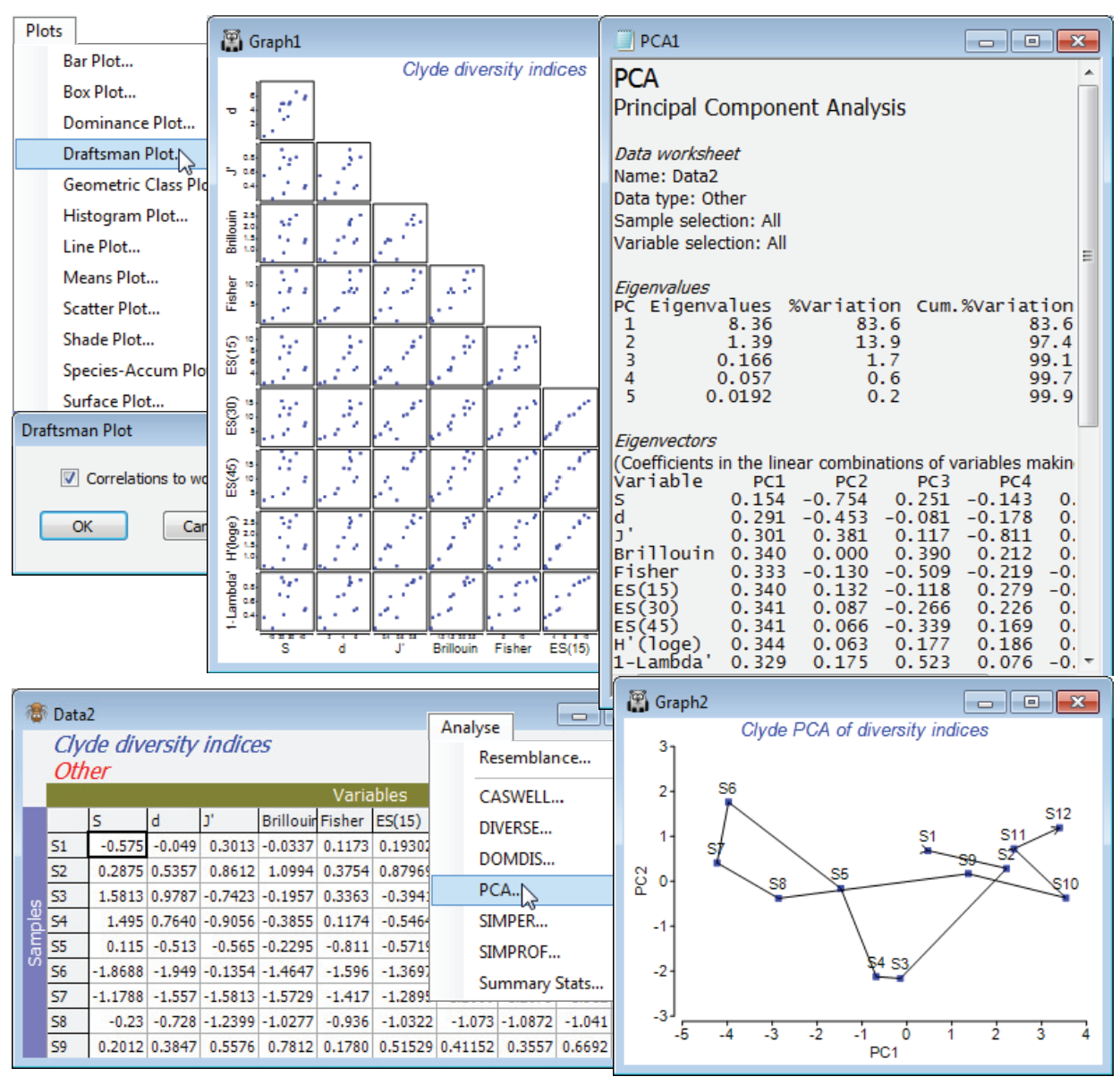
For the diversity (variables) by samples matrix, Data1, **Plots>Draftsman Plot**>(✓Correlations to worksheet) shows that none of the indices is badly behaved, i.e. skewed, dominated by outliers, strongly curvilinear relationships etc., so no transforms seem called for. \[To get the plot below, you might find it helpful to increase the symbol size on the **Samp. labels & symbols** tab, and on the **X & Y axis** tabs increase the title font sizes, unchecking (✓Limit size)\]. Data1 needs **Pre-treatment>Normalise Variables**, however, before entry to **Analyse>PCA** since the indices are on different scales. On the configuration plot from PCA, turn off (✓Overlay vectors) on **Special>Overlays** and instead (✓Overlay trajectory) of the transect Site#. Site 6 is the dumpground centre, with Sites 1 and 12 at the extremities of the transect, and this combined set of diversity indices clearly displays the strong, simple gradient of effect, in a rather similar way to the full multivariate analysis of the original species data (you might like to carry out the latter, with a fairly severe transformation and Bray-Curtis similarities). The agreement is a consequence of the severity of the impact. The *meta-analysis* of Chapter 15 of CiMC shows this to be the most severe of the contaminant studies looked at there, but Chapter 14 also shows that such agreement is untypical, diversity measures being less likely to detect biological change for more intermediate-level disturbances. The PCA results (the eigenvalues) also make it clear that rather little is to be gained by calculating ten diversity indices instead of two or three: over 83% of the total variation in the 10 indices is accounted for by the first PC, and 97% (i.e. all of it, in effect) by the first two PC’s. The coefficients (eigenvectors) show that the simple left to right gradient in the main axis (PC1) of the PCA is a roughly equally weighted combination of all measures (evenness + richness), both increasing away from the dumpground, whereas the second axis strongly contrasts the two main diversity components: PC2 is effectively (evenness – richness). This simplicity should not be a surprise, given the high correlations between indices evident from the draftsman plot, and from the correlation matrix Resem1 created with it.
[](https://learninghub.primer-e.com/uploads/images/gallery/2024-10/screenshotpage267a.png)
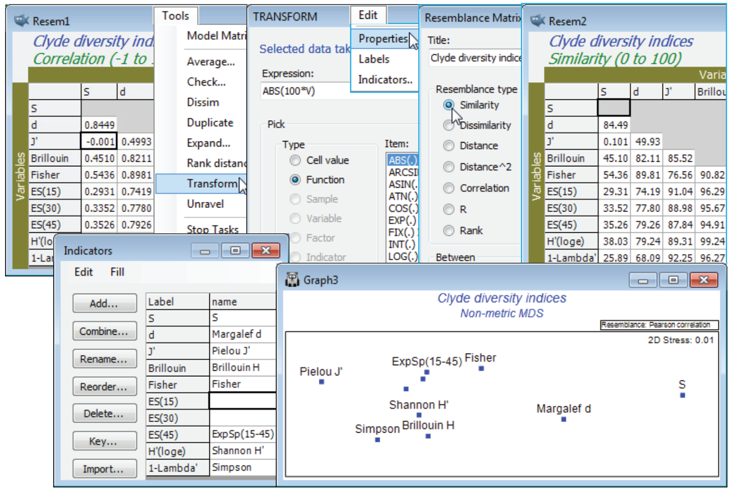
A final, revealing plot can be produced from Resem1, by ordinating the variables. Technically, it first needs transforming before it can be considered a similarity matrix: there is a small, negative correlation between *S* and *J*$^{\hspace{2pt} \prime}$. It is effectively zero here, but other situations might produce large negative correlations, e.g. between equitability and dominance measures, and they should also imply similarity (of variables). **Tools>Transform**>(Expression: 100*ABS(V)) on Resem1 will achieve the conversion to a similarity matrix (and you could change its type on **Edit>Properties**). Then **Analyse>MDS>Non-metric MDS (nMDS)** generates the ordination plot for the variables shown below, in which the relative distances apart of the indices exactly reflects the rank order of their pairwise correlations (note that the MDS stress is effectively zero). The plot is largely linear, the extremities corresponding to pure richness (*S*) and evenness (*J*$^{\hspace{2pt} \prime}$), with other measures being a mix of these two components. The points have been more descriptively labelled using **Var. labels & symbols**>(Labels✓By indicator)>**Edit**, which is equivalent to **Edit>Indicators** on the Resem1 sheet, then **Add** an indicator: name. The boundary of the *n*MDS plot has also been appropriately reshaped for this linear plot, with **Special>Main**>(Plot type•2D>Aspect ratio: 3). Values of *n* = 15, 30 and 45 were chosen for the rarefaction indices *ES(n)* because larger values are not permissible, the site with lowest abundance having only 46 individuals. (To see this **Analyse>Summary Stats**>(For•Samples)>(✓Sum) on Clyde macrofauna counts, or just ask for ✓N in **Analyse>DIVERSE**). The fact that the *expected species numbers ES(n)* are clearly considerably closer to being evenness measures than the richness indices that their name implies (correlations of about 0.9 with *J*$^{\hspace{2pt} \prime}$ and 0.98 with *H*$^{\hspace{2pt} \prime}$, compared with about 0.3 with *S*) results from the lack of ecological realism in their underpinning model. This assumes that individuals arrive randomly and independently into the sample, and hence the process can be reversed in rarefaction, by randomly excluding them. This does not correspond to the reality of a clumped spatial distribution seen for many species (as seen in Dispersion Weighting, Section [4](https://learninghub.primer-e.com/books/primer-v7-user-manual-tutorial/chapter/4-pre-treatment-options)). Resave the workspace Clyde ws2 for later use, and close it.
[](https://learninghub.primer-e.com/uploads/images/gallery/2024-10/screenshotpage268a.png)