# Other 1-way ANOSIM options
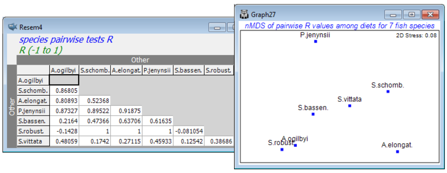
Checking the (✓Pairwise tests to worksheet) box has also sent the above R values to a worksheet in triangular format, which could be a useful layout for tabulating ANOSIM results in a publication. More subtly, this can be regarded as a resemblance matrix (of distance-type) in its own right – the higher the value of R the greater the separation of replicates from two groups in the high-d (prey) space. Inputting this to an MDS plot will display the relationships between these 7 groups, and can be seen as a type of means plot. \[Note that this triangular array is not a sensible distance matrix at present because it can, and does, contain (small) negative values. Input to metric MDS without some prior rescaling would be problematic therefore. However, *n*MDS effectively works only on the rank orders of the entries so there is no need to rescale them – the lowest values (the negative ones) indicate the least established differences in diet and the highest values (R=1) the greatest differences, which is exactly what is required for a sensible *n*MDS plot here. Dropping the negative signs, by taking absolute values of the entries, would not be the technically correct approach here.\]
The more straightforward means plots, as we have seen before, is to average the replicates, and then calculate Bray-Curtis between these mean dietary samples, ordinating by *n*MDS or *m*MDS. But there are many other possibilities for a direct means plot! The data could be transformed before or after averaging, or the dissimilarities could be averaged – or even their ranks averaged. PRIMER 7 now has the option to average (dis)similarities across a group structure, with **Tools>Average** for an active window of a resemblance matrix. **Tools>Rank distance** will also replace resemblance entries with their ranks. (A further option is given in the PERMANOVA+ add-on, of computing *distances among centroids* in the high-d PCO space formed from the resemblance matrix). These will all give means plots with slightly different emphases. In the case of the matrix of R values, this highlights relative group separations, i.e. adjusting differences by within-group dispersion.
[](https://learninghub.primer-e.com/uploads/images/gallery/2024-07/screenshotpage154a.png)
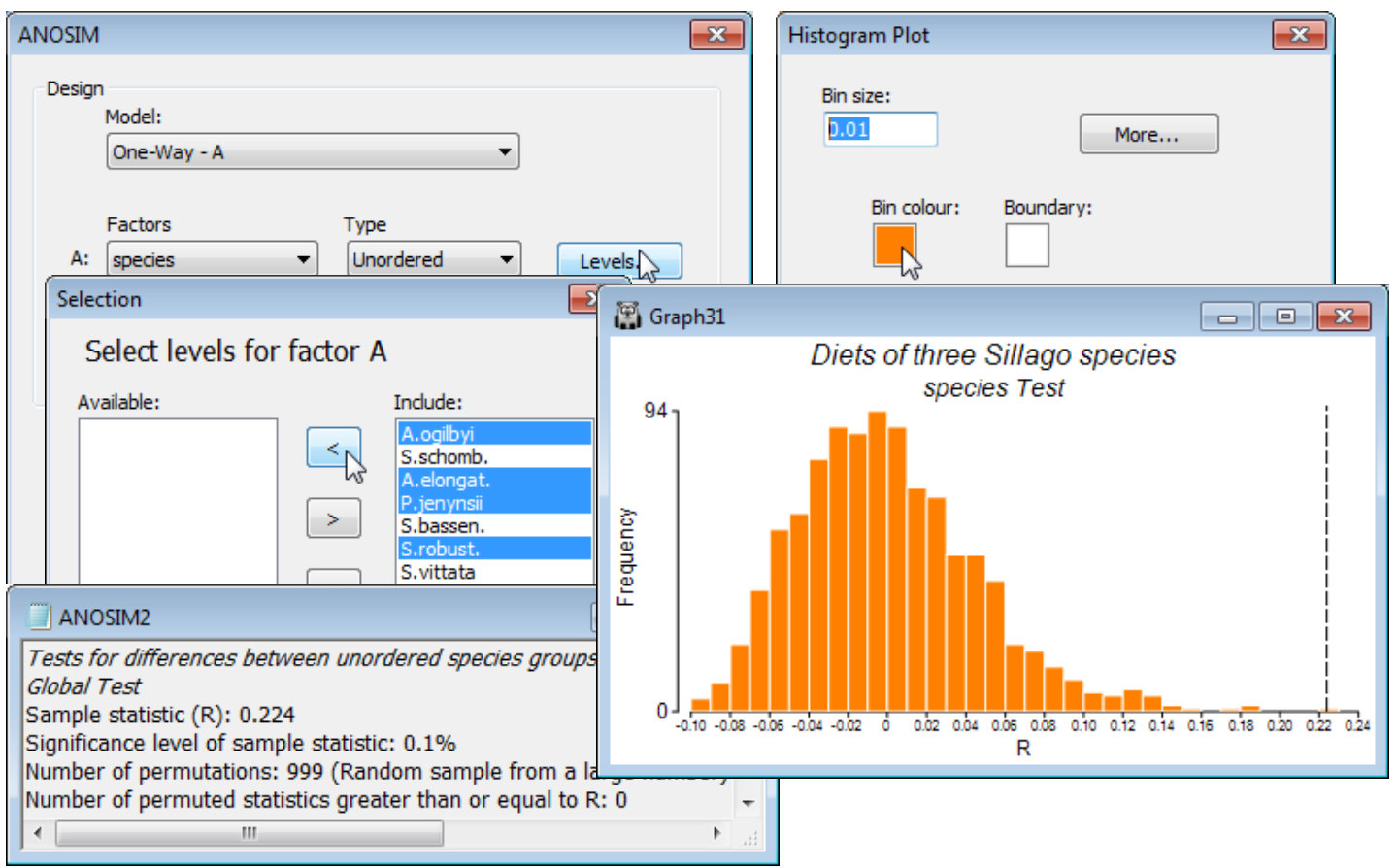
Other options within the ANOSIM routine include the ability to manipulate the histogram for the global R statistic by rescaling axes, titles etc. (the usual **Graph>Sample Labels & Symbols** menu) and changing bin widths and, in v7, bin colours (**Graph>Special**), as for any other histogram plot. There is also a check box in the ANOSIM dialog to send (✓R values to file). You would then need to supply an \*.txt file name which will hold a simple list – one number to a line, in simple text – of the R values for the 999 (or however many) permutations carried out for the global test. This would allow the null distribution data to be replotted, for example, in another statistical/graphical package.
As noted earlier, the plotted histogram (and the listed R values) refer only to the global test for no differences among any of the groups. If you require a histogram for a specific pairwise comparison then you will need to pick out that pair of groups and re-run **ANOSIM**, selecting either externally, by **Select>Samples** on the original resemblance matrix, or internally, using the **Levels** button for A on the ANOSIM dialog. Both lead to the usual Selection dialog. For a pairwise test, it will make no difference to the R value (or to its significance level) whether the results are read from the above pairwise table or recalculated with just those groups selected, so this would only be useful: a) if you required the pairwise histogram, or b) a test for a specific subset of three groups, four groups etc. was needed. As seen in Section [3](https://learninghub.primer-e.com/books/primer-v7-user-manual-tutorial/chapter/3-highlighting-and-selection-select), a relevant *a priori* hypothesis here concerns whether there are detectable dietary differences between the three congeneric *Sillago* fish species (*S. schomburgkii*, *S. bassensis* and *S. vittata*). After testing this, save and close the workspace WA fish ws.
[](https://learninghub.primer-e.com/uploads/images/gallery/2024-07/screenshotpage155a.png)