# Other Model Matrix options
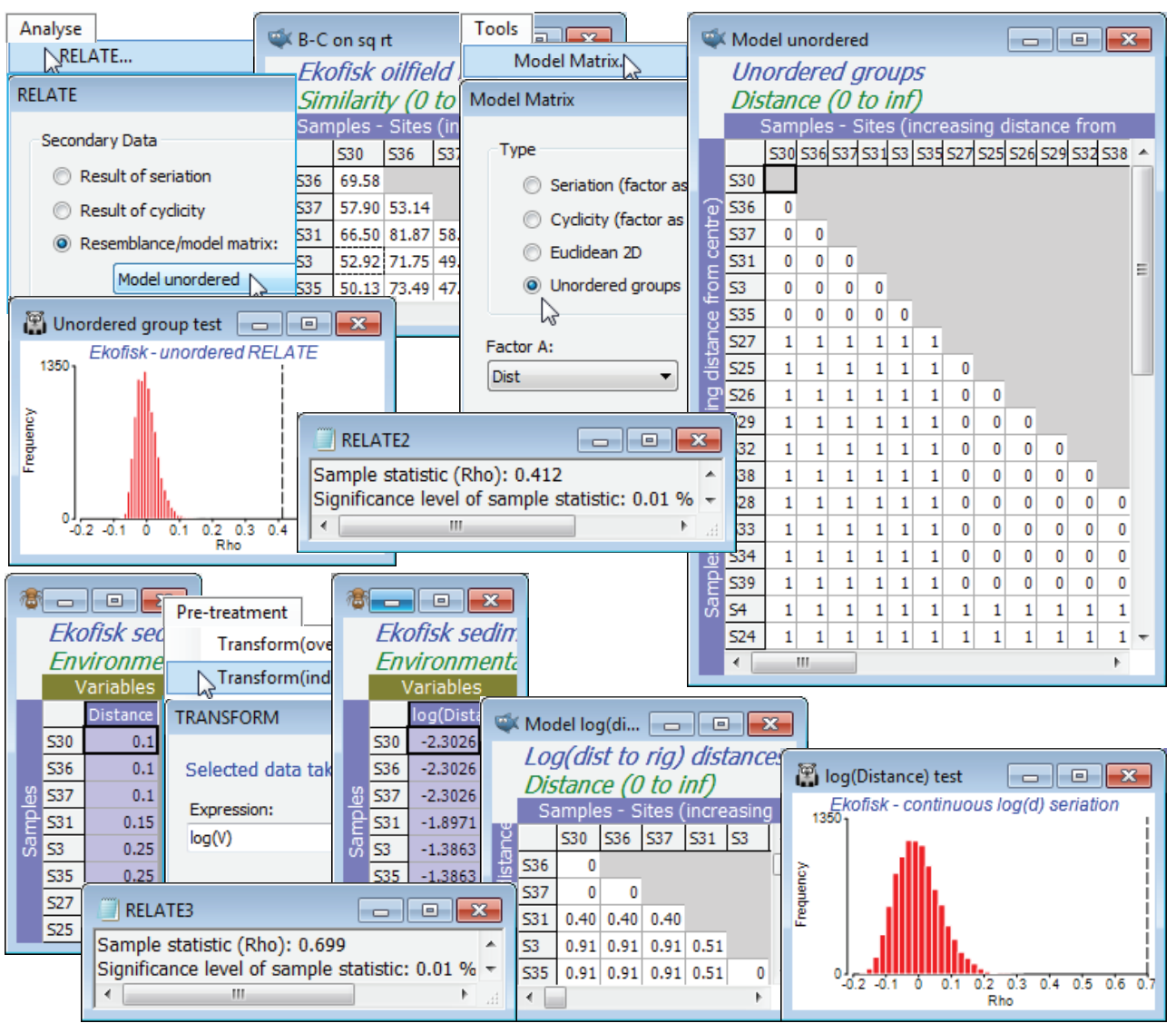
The conclusion is, of course, consistent with the different, but closely-related, ordered ANOSIM statistic R$^{\text Oc}$ = 0.67 (p<0.01%), calculated in Section [9](https://learninghub.primer-e.com/books/primer-v7-user-manual-tutorial/chapter/9-analysis-of-similarity-tests-unordered-and-ordered-anosim). It is relatively easy to show algebraically that the unordered ANOSIM statistic – here R = 0.55, with p<0.01% again – is exactly equivalent (see Chapter 6 of CiMC) to a RELATE $\rho$ test with model matrix having 0’s in the diagonal blocks (samples within the same group) and 1’s elsewhere (samples in different groups), i.e. all groups are considered equally different from each other. Such a model matrix can be constructed by **Tools>Model Matrix**>(Type•Unordered groups) & (Factor A: Dist) – or (Factor A: Dist#), since it no longer matters whether an unordered factor is supplied as numeric or alphabetic. This test returns $\rho$ = 0.41, again strongly significant, naturally, but much lower than the seriation statistic $\rho$ = 0.63.
So far we have not seen anything that could not have been slightly better carried out with ordered and unordered ANOSIM tests (in the sense that the statistic upper limit of +1 is attainable for R$^{\text O}$ but not for $\rho$ – see Chapter 6 of CiMC – and because ANOSIM will allow pairwise comparisons among the groups). But another possible model here which we would like a comparison with – one which can only be handled by RELATE – is to ignore the arbitrary distance group structure and RELATE the biotic similarities to the distance matrix calculated from (log-transformed) distances of each site to the oilfield centre. (The log transform reverses an exponentially decreasing dilution curve of contaminant concentrations with distance). The raw distances are in the first column in the abiotic sheet Ekofisk environment, the *Distance* variable (you may need to **Select>All** to find it!). Highlight and select just this column, log transform it by **Pre-treatment>Transform(individual)**> (Expression: log(V)) and **Analyse>Resemblance**>(Measure•Euclidean distance), renaming the result as Model log(distance) and inputting it as the secondary matrix to an **Analyse>RELATE** on B-C on sq rt. The result is again significant, naturally, but arguably demonstrates an even stronger gradient of assemblage change with this model of continuous (logged) distance from the oilfield, $\rho$ = 0.70 (p<0.01%). This model matrix could also have been created by copying the log(Distance) entries into a factor log(D) under the B-C on sq rt resemblance sheet and running **Tools>Model Matrix**>(Type•Seriation (factor as distance)) & (Factor A: log(D)). Save and close Ekofisk ws.
[](https://learninghub.primer-e.com/uploads/images/gallery/2024-10/screenshotpage246apng.png)