# Ranked variables
The following section (on PCA) will discuss further the choice of particular transformations to avoid the sensitivity of PCA (and Euclidean distances in general) to outliers in some environmental variables, but choice of individual transformations is often a worry to practitioners. An alternative, eliminating the need for choice (but arguably losing some sensitivity in the ensuing analysis), is to replace variables by their ranks, namely the numbers 1, 2, 3, … for largest to smallest values across samples (modified if necessary to substitute average ranks for tied values). The main advantage is that the over-dominant contribution of outliers is automatically eliminated. For example, a variable whose values over the samples, in decreasing order, are: 25, 9, 7, 6, 6, 6, 4, 2, 2, 0 would generate ranks: 1, 2, 3, 5, 5, 5, 7, 8.5, 8.5, 10 respectively, and the effect is to make the outlying value of 25 no different than if it had been 15 or 10. Ranking each variable (separately) also removes the need for normalising the resulting array, which is needed (after transformation) with the usual approach, to ensure that all environmental variables take values across comparable ranges. Ranking places all variables on a common measurement scale, the numbers 1 to *n* (where *n* is the number of samples).
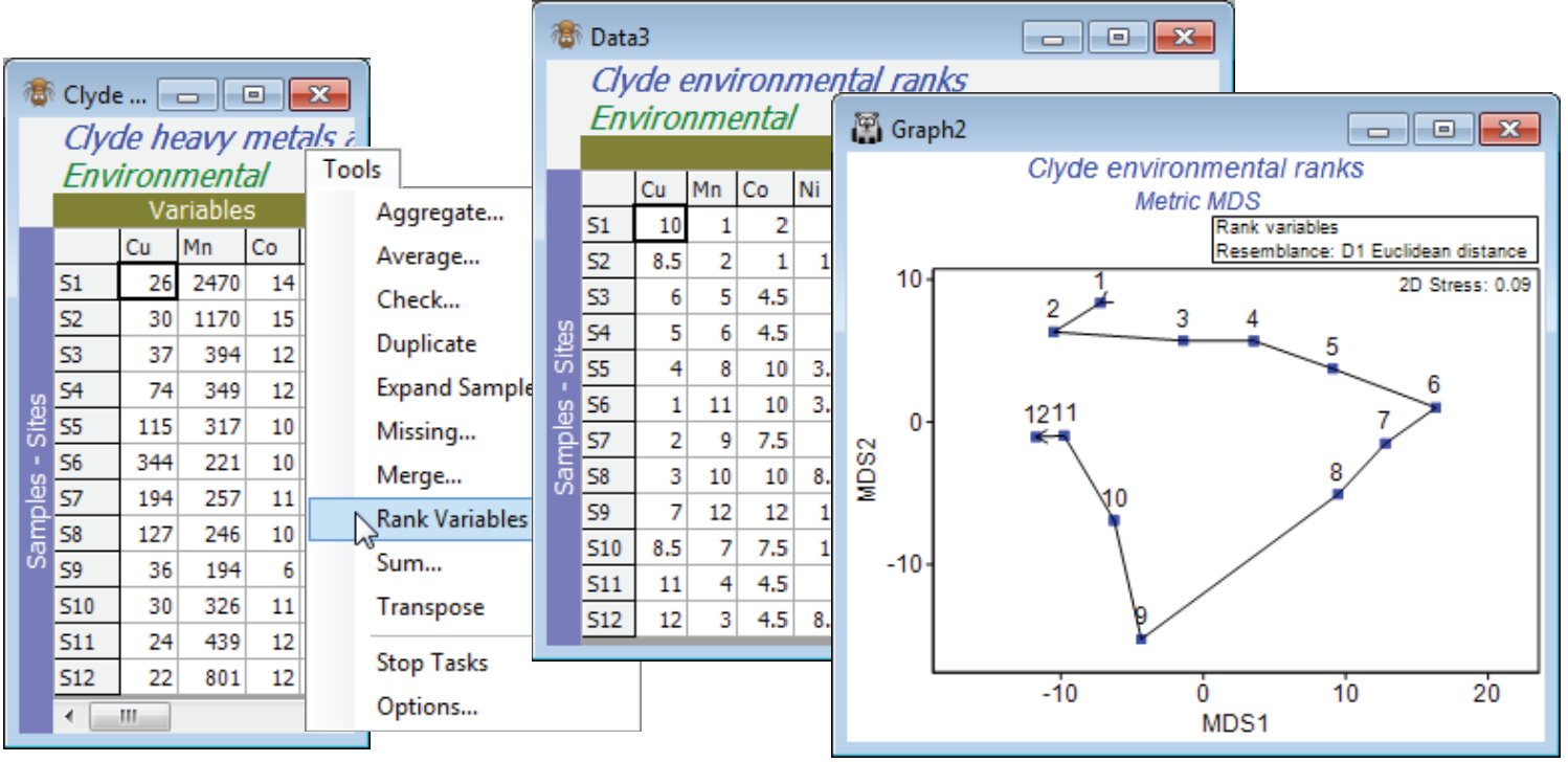
For the original (complete) Clyde environment sheet, take **Tools>Rank variables** and examine the outcome. Put this matrix through **Analyse>Resemblance**>(Measure•Euclidean distance) and then **Analyse>MDS** for a non-metric or metric MDS (the latter has a better chance of being acceptable because of the few points and the simple gradient structure, and importantly, the Euclidean distance matrix). In order to overlay a trajectory on the MDS with **Graph>Special>Overlays**>(✓Overlay trajectory)>(Trajectory numeric factor: Site#), you will need either to create the *Site#* factor for any sheet on the Clyde environment branch, with **Edit>Factors>Add**>(Add factor name: Site#), highlighting the column and **Fill>Label number**, to generate the values 1 to 12. (Alternatively, if you have already opened the abundance file Clyde macrofauna counts into the workspace, you can **Factors>Import** the factor *Site#* from that sheet). It is interesting to note the linearity of Shepard diagrams for both *m*MDS and *n*MDS but whilst the ordinations look very similar, the *m*MDS fit of a straight line through the origin is not quite such a good fit (stress = 0.09 c.f. *n*MDS stress = 0.03). The main point here, though, is that this ordination, based on ranked data, looks very similar to the PCA which we shall see in Section [12](https://learninghub.primer-e.com/books/primer-v7-user-manual-tutorial/chapter/12-analysing-environmental-variables-draftsman-plot-pca), based on transformation and normalisation of this data.
[](https://learninghub.primer-e.com/uploads/images/gallery/2024-09/screenshotpage215a.png)