# Running Type 2 SIMPROF
A Type 2 SIMPROF test is not part of a **Wizards>Coherent plots** run, and there is a good case for carrying out a test of its null hypothesis \(H$_0$: there are no species associations at all\) prior to trying to break down those associations into coherent groups, i.e. within each group the null hypothesis (H$_0$: all species similarities within a group are the same) cannot be rejected. Inclusion of species with so little information that species similarities (index of association, IA) are totally unreliable is again unhelpful, so we start from the matrix reduced to the 50 ‘most important’ species. For this test (Type 2), it does not make any difference whether we use the selection in Data1 or its species-standardised form Data2, because the permutations will be across samples within each species and IA includes a standardisation step in its formula. (It does, however, matter a great deal to use the standardised form Data2 when carrying out Type 3 SIMPROF tests – either as part of clustering or with **Analyse>SIMPROF** – because permutations are across species within samples, and this will make no sense if species are not first ‘relativised’ in this way, to total 100% over samples).
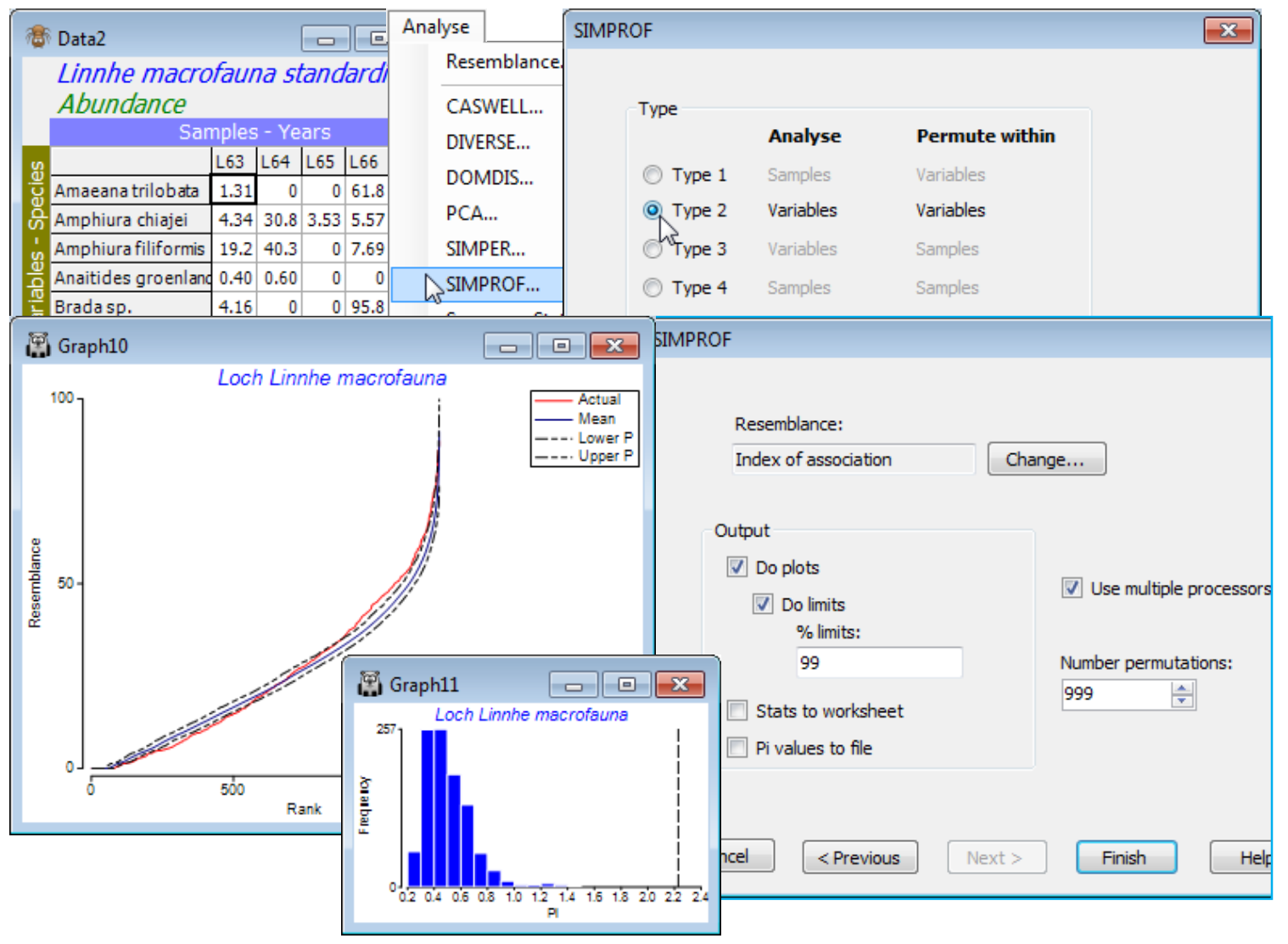
So, from the selection in Data1 or from Data2, run **Analyse>SIMPROF**>(Type•Type 2) and take the defaults on the **Next** screen. The output, *MultiPlot2*, contains two graphs, of the real similarity profile (red) and the means and 99% probability limits for that profile under the null hypothesis, and the histogram of absolute deviations $\pi$ of 999 (further) permuted profiles from that mean, with the real statistic value $\pi$ indicated by the dotted vertical line. The output is of exactly the same form as previously discussed for single **SIMPROF** runs (see Section [6](https://learninghub.primer-e.com/books/primer-v7-user-manual-tutorial/chapter/6-clustering-methods-cluster-simprof-unctree-krcluster)), and shows with little doubt that there are real species associations to interpret (p<0.1%). With a large number of similarities making up the profile (50$\times$49/2 = 1225), it is inevitable that the probability limits and the real profile will hug the mean curve fairly closely but it is clear that there is an excess of both higher and lower associations than one would expect by chance under the null hypothesis – some of the species are ‘positively’ associated and some ‘negatively’ (we retain the terminology of correlations being positive or negative though, as explained in Chapter 7 of CiMC, an index of association defined over (0, 100) is a better measure of species inter-relationships than a correlation coefficient). Note that very few of the ‘negative’ associations are at the lower limit of IA = 0, which arises when two species are only ever found in different years – this is the result of removing all the low abundance species. \[About half the original 111 species were found in three or fewer years – and if you prefer to carry out a species reduction on this type of criterion, you can do so by **Select>Variables**>(In at least n samples where n is ), entering that reduced matrix to **Analyse>SIMPROF** and **Wizards> Coherence plots**. Leaving in rare species always results in a tail of fully ‘negative’ associations.\]
[](https://learninghub.primer-e.com/uploads/images/gallery/2024-08/screenshotpage193a.png)