# Standard indices calculated
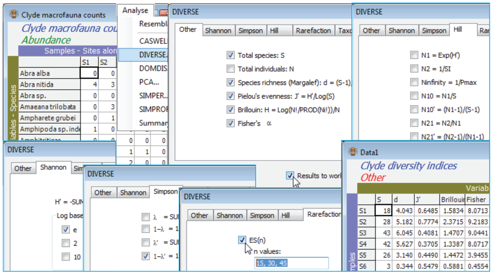
The range of indices available is illustrated with the macrobenthic data Clyde macrofauna counts from the Clyde sludge dump-ground study, directory C:\Examples v7\Clyde macrofauna, last seen in Section [14](https://learninghub.primer-e.com/books/primer-v7-user-manual-tutorial/chapter/14-further-matching-of-multivariate-patterns-relate-2stage-best-mvdisp). Analyses so far have used only the abiotic and biomass matrices, and the existing workspace Clyde ws may have become cluttered, so open Clyde macrofauna counts into a new workspace, and save it as Clyde ws2. Without pre-treatment, take **Analyse>DIVERSE**>(✓Results to worksheet). Look at the options on the first 5 tabs, taking only ✓S, ✓d, ✓J$^\prime$, ✓H, ✓$\alpha$, ✓H$^\prime$ (log base e), ✓1 – $\lambda^\prime$, ✓ES(n) with n values: 15, 30, 45 (there is no special significance to the index grouping under tabs, except that the last two tabs deal with taxonomic-relatedness measures, seen later). The abundance of the *i*th species is denoted by N$_i$ (*i* = 1, 2, .., S) and, as a ratio of their sum (*N*), this is denoted P$_i$ (*i* = 1, 2, .., S). The first 5 tabs (where ✓ denotes the default selections) are:
**Other**
✓Total species: $S$
✓Total individuals: $N$
✓Species richness (Margalef): $d = (S – 1)/\log_e N$
✓Pielou’s evenness: $J^\prime = H^\prime / \log_e S$
Brillouin: $H = N^{-1} \log_e \\{ N! / (N_1!N_2!…N_S! ) \\} $
Fisher’s $\alpha$ statistic
**Shannon**
✓$H^\prime = – \sum P_i \log(P_i)$, where the logs are to the base e
$H^\prime$ as above but for logs to the base 2
$H^\prime$ as above but for logs to the base 10
**Simpson**
$\lambda= \sum P_i^2$
$1 - \lambda= 1- (\sum P_i^2)$
$\lambda^\prime= \\{ \sum_i N_i (N_i–1)\\} / \\{N(N–1) \\}$
✓$1-\lambda^\prime= 1- \\{ \sum_i N_i (N_i–1)\\} / \\{N(N–1) \\}$
**Hill** numbers
$N1 = \exp (H^\prime)$
$N2 = 1/ \sum P_i^2$
$N_ \infty = 1/ \max_i \\{P_i\\}$
$N_{10} = N1/S$
${N_{10}}^\prime = (N1–1)/(S–1)$
$N_{21} = N2/N1$
${N_{21}}^\prime = (N2-1)/(N1-1)$
**Rarefaction** (Sanders/Hurlbert)
$ES_n$, the ‘expected’ number of species from $n$ individuals ($n \le N$)
[](https://learninghub.primer-e.com/uploads/images/gallery/2024-10/screenshotpage266a.png)