# (Tikus Island coral cover)

Data on coral communities at a site in Tikus Island, Thousand Islands, Indonesia, over the years 1981, 83, 84, 85, 87 and 88, were reported by Warwick RM, Clarke KR, Suharsono 1990, *Coral Reefs* 8: 171-179. Ten replicate transects were examined each year, and the data is the length of intersection of a transect (as a percentage of transect total length) by each of the 58 coral species identified, file <ins>Tikus coral cover</ins> in directory C:\Examples v7\Tikus corals. The region was subject to a coral bleaching event in 1982 (probably El Niño related), so that the 1983 samples are very denuded of live coral – this is a classic situation in which a zero-adjusted Bray-Curtis similarity is likely to be useful, and this example is discussed in detail in the Clarke *et al* 2006 paper mentioned above. A dummy value of 1 is a natural choice here because the smallest non-zero entries for each species are about 1%, or marginally less. To see these entries, highlight the whole array, take say **Pre-treatment>Transform(individual)**>(Expression:<ins>V-10*(V=0)</ins>) and enter the resulting sheet to **Analyse>Summary Stats**>(For•Variables)&(✓Minimum). This works because the BASIC syntax expression computed on the value V in every cell, <ins>V-10*(V=0)</ins>, returns either -1 (true) or 0 (false) for V=0, multiplies this up to -10 or 0, so when subtracted from V returns +10 in any cell which is zero and leaves non-zero values alone. **Summary Stats** then finds the minimum for each species. (10 in the expression could be replaced by any large number). If you run the Summary Stats again, this time (For•Samples)&(✓Minimum) you will get the lowest non-zero entry in the whole matrix.

[![ScreenshotPage66a.png](https://learninghub.primer-e.com/uploads/images/gallery/2024-05/scaled-1680-/screenshotpage66a.png)](https://learninghub.primer-e.com/uploads/images/gallery/2024-05/screenshotpage66a.png)

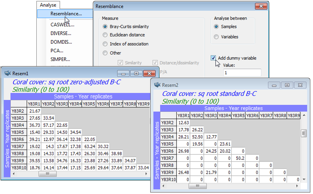
As in the previous section, **Plots>Shade Plot** readily shows that a (mild) square root transform is necessary to avoid the resemblance calculation being dominated by just a couple of species with occasionally very large %cover values. So, after **Pre-treatment>Transform(overall)**><ins>Square root</ins>, take **Analyse>Resemblance**>(Measure•Bray-Curtis similarity) & (Analyse between•Samples) & (✓Add dummy variable>Value: <ins>1</ins>), this dummy value of 1 being equally suitable after any power transformation or reduction to presence/absence (1/0). By repeating this calculation on the square-rooted data, but without the dummy variable, a quick glance at the two resemblance matrices shows the dramatic effect of the zero-adjustment here, e.g. among the 1983 replicates. (This translates into substantial differences in the clustering, MDS ordination, ANOSIM tests etc, see Fig. 16.7, CiMC). **File>Save Workspace As**>(File name:<ins>Tikus ws</ins>) in the C:\Examples v7\Tikus corals directory.

[![ScreenshotPage68a.png](https://learninghub.primer-e.com/uploads/images/gallery/2024-06/scaled-1680-/screenshotpage68a.png)](https://learninghub.primer-e.com/uploads/images/gallery/2024-06/screenshotpage68a.png)