# (W Australia fish diets)

The diet study for 7 species of W Australian fish, with a variable number of dietary samples from each, has been seen several times now. In Section [3](https://learninghub.primer-e.com/books/primer-v7-user-manual-tutorial/chapter/3-highlighting-and-selection-select) we selected a subset of just the 3 congeneric species, *Sillago schomburgkii* (10 samples), *S. bassensis* (14) and *S. vittata* (16), labelled as B, E and G, and decided to omit samples B3 and B4 from these species (and also A9 from *A. ogilbyi*) on grounds of very much lower total gut content than other samples. In Section [4](https://learninghub.primer-e.com/books/primer-v7-user-manual-tutorial/chapter/4-pre-treatment-options), we noted that it was necessary to standardise these samples across the 32 prey categories (the ‘species’ variables) since total gut content  of a sample (units are %volume) could not be controlled – since the fish are doing the sampling(!) – and differences in these totals are of no relevance in seeking dietary distinctions among these 3 closely-related species. In Section [8](https://learninghub.primer-e.com/books/primer-v7-user-manual-tutorial/chapter/8-multi-dimensional-scaling-non-metric-nmds-metric-mmds-combined-mds), we looked at *n*MDS plots for all 7 fish species in higher-dimensions since a 2-d plot had high stress, and noted the differences in variability in diet among the species, and in section [9](https://learninghub.primer-e.com/books/primer-v7-user-manual-tutorial/chapter/9-analysis-of-similarity-tests-unordered-and-ordered-anosim), we ran the ANOSIM global and pairwise tests between the species to establish the statistical significance (or otherwise) of dietary differences. In Section [10](https://learninghub.primer-e.com/books/primer-v7-user-manual-tutorial/chapter/10-wizards-and-species-analyses-basic-mva-coherence-plots-matrix-display-simper) we referred to use of SIMPER to identify the main dietary categories accounting for dissimilarity among fish species, where these were established with confidence by the ANOSIM tests (and shade plots would also be instructive here). Previously, towards the end of Section [8](https://learninghub.primer-e.com/books/primer-v7-user-manual-tutorial/chapter/8-multi-dimensional-scaling-non-metric-nmds-metric-mmds-combined-mds), we had shown some of those dietary categories on the 3-d *n*MDS of the samples, in a 3-d bubble plot, and also gave a means plot, averaging over the samples for each of the 7 fish species – on this we then displayed a segmented bubble plot of the main prey categories distinguishing the diets. We can now fit one final small piece to this jigsaw, by adding bootstrap regions to the means plot. In fact, it would be unwise to attempt this for the full set of species, since three of them have only 3, 4 and 5 replicate samples and the motivating concept of bootstrapping (generating ‘other sets of means we could have observed’) is more or less certain to break down with such small replicate numbers – the sampling with replacement just does not produce enough realistically different combinations, see Chapter 18 of CiMC, to avoid major underestimation of the true variation in those means. A fourth species, *A. ogilbyi* does have plenty of replicates and could be included (and you could do so), but for this illustration we look again at a logical subset – the three congeneric *Sillago* species – and construct an *m*MDS plot with bootstrap regions for their average dietary assemblages.

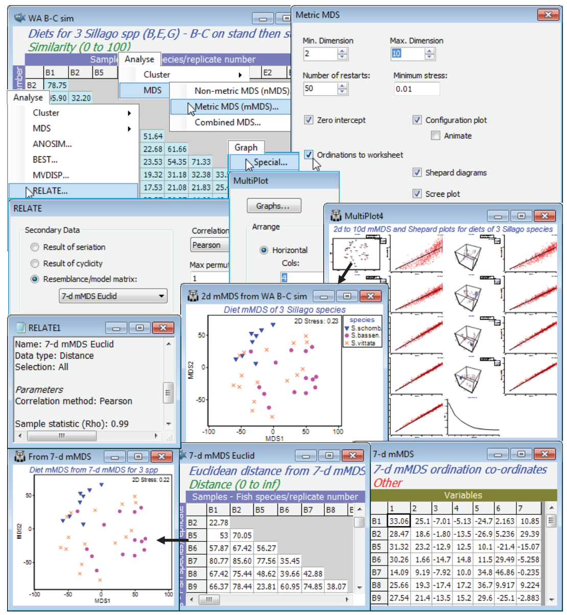
Open workspace <ins>WA fish ws</ins> from C:\Examples v7\WA fish diets, which should contain the resemblance matrix <ins>WA B-C sim</ins> for all samples (excluding A9, B3 and B4) of the 7 fish species. If not available, you will have to repeat the earlier steps of: opening the data file <ins>WA fish diets %vol</ins>, deselecting A9, B3, B4, standardising samples by total (**Pre-treatment>Standardise**), square root transforming and computing Bray-Curtis, renaming this <ins>WA B-C sim</ins>. Now highlight and select from this just the B, E and G labels – or instead **Select>Samples**>(•Factor levels)>(Factor name: <ins>species</ins>)>**Levels**>(Include: <ins>S.schomb.</ins>, <ins>S.bassen.</ins>, <ins>S.vittata</ins>). On these selected resemblances, run **Analyse>MDS>Metric MDS(mMDS)**>(Min. dimension <ins>2</ins>) & (Max. dimension <ins>10</ins>), taking other defaults such as (✓Zero intercept), but <u>adding</u> (✓Scree plot) and (✓Ordinations to worksheet). On the multi-plot this produces, reform the rows/columns by **Graph>Special**>(Arrange•Horizontal) >(Cols: <ins>4</ins>). By clicking on individual plots within this multi-plot, note how the 2-d *m*MDS is of relatively high stress for the (only) 38 samples – as noted earlier, *m*MDS stress values will always be higher than for the equivalent *n*MDS but the Shepard diagram for the 2-d plot is also not very convincing. This changes, however, for higher dimensional solutions, with the Shepard diagrams becoming increasingly well described by a straight line through the origin (read across rows of the multi-plot for the Shepard diagrams in dimensions: 2 & 3, 4 & 5, 6 & 7, 8 & 9, 10 & the scree plot). By the time this gets as far as about a 7-dimensional *m*MDS solution, the stress has reduced to 0.03-0.04 – a very low stress for a metric MDS plot, capturing the original dissimilarities (not just their rank orders) to a high precision in the (Euclidean) distances between co-ordinate points in the 7-d *m*MDS plots. In fact, it is worth seeing that if you repeat the above 2-d *m*MDS, but this time starting from those Euclidean distances in 7-d *m*MDS space, the 2-d ordination appears to be identical to that produced from the original Bray-Curtis similarities for these three species. \[You obtain these Euclidean distances by finding the data sheet containing the 7-d co-ordinates from your original *m*MDS run – because the (✓Ordinations to worksheet) instruction has sent 9 further sheets to the Explorer tree, of the 10-d down to the 2-d *m*MDS co-ordinates – then simply enter that 7-d co-ordinate data to **Analyse>Resemblance**>(•Euclidean distance), giving <ins>7-d mMDS Euclid</ins>\]. Of more relevance to understanding the bootstrap methodology, however, is to calculate (not test) the **Analyse>RELATE** statistic on the original similarities, <ins>WA B-C sim</ins>, with (•Resemblance/ model matrix: <ins>7-d mMDS Euclid</ins>) & (Correlation method: <ins>Pearson</ins>), which returns $\rho$= 0.99. 

[![ScreenshotPage291a.png](https://learninghub.primer-e.com/uploads/images/gallery/2024-11/scaled-1680-/screenshotpage291a.png)](https://learninghub.primer-e.com/uploads/images/gallery/2024-11/screenshotpage291a.png)