Should I use PRIMER or R?
Use both! They are good at different things. by Marti J. Anderson (2024)
- Citation
- 1. Let's consider using PRIMER
- 2. Let's consider using R
- 3. PERMANOVA vs adonis2 in R
- 3.1 Compare example output
- 3.2 Results don't match
- 3.3 How does PERMANOVA do it?
- 3.4 How does adonis2 do it?
- 3.5 What about $R^2$ values?
- 3.6 Summarising the comparison
- 4. Take-home messages
- 5. References
Citation
Anderson, M.J. (2024) Should I use PRIMER or R? PRIMER-e Learning Hub. PRIMER-e, Auckland, New Zealand. https://learninghub.primer-e.com/books/should-i-use-primer-or-r.
1. Let's consider using PRIMER
1.1 PRIMER has a lot going for it
PRIMER has a special focus - robust multivariate methods
PRIMER is a specialised piece of software that is purposefully designed to analyse multivariate data. It is especially good at handling high-dimensional, non-normal data, which are not able to be analysed using classical multivariate statistical methods.
Non-normal high-dimensional data arise commonly in community ecology and environmental science, where abundances (counts, biomass, presence/absence or cover values) of individual species are sampled. They also arise in a lot of other contexts.
Many of the routines in PRIMER implement statistical or graphical methods that rely flexibly on a similarity (or dissimilarity or distance) matrix among sample units (or variables), or their ranks, as a fundamental foundation. The statistical methods and tests in PRIMER are very robust. They use carefully constructed permutation algorithms to ensure all tests are valid and distribution-free. The initial suite of non-parametric methods in the PRIMER base package (e.g., ANOSIM, RELATE, BEST, MDS, SIMPROF, LINKTREE, TAXDTEST, etc.) are further extended by a suite of semi-parametric methods offered in the PERMANOVA+ add-on package for PRIMER (e.g., PERMANOVA, PERMDISP, dbRDA, DISTLM, CAP, etc.), enhancing the overall capability of PRIMER software.
PRIMER (and PERMANOVA+) arose in response to (mostly marine) scientists, to service a clear need to analyse ecological community data. However, the methods are sufficiently general, robust and flexible to accommodate multivariate data in virtually any applied setting (e.g., genetics, economics, psychology, medicine, agriculture, etc.). This has led to the broad use and popularity of PRIMER/PERMANOVA+ software globally as a useful general tool for performing robust multivariate analysis.
PRIMER is extremely easy to use
PRIMER is very easy to use (point and click). It operates in a Windows GUI that is familiar, straightforward and intuitive. You don’t have to program anything or write any code. You never have to worry about de-bugging the engines underneath the user interface. Data types are explicit and clear, on input.
In addition, PRIMER offers some tailored error messaging that can assist you to make sensible decisions along your statistical analysis pathway, given the type of data you are working with. Of course, you have full control and can bypass suggestions or defaults offered by the package, but those who are new to PRIMER (and those of us who are old hands!) are helpfully supported by these features.
PRIMER also has some tailored 'Wizards' to make data import and other multi-task analysis pipelines quicker and easier to achieve. This leaves you more time to concentrate on the results and your interpretation, instead of struggling with code.
Ease-of-use also makes it super quick to trial a host of different approaches on a single (or multiple) sets of data, without losing track of your core purpose. Everything is kept within a single file (a PRIMER workspace, *.pwk), and you can even add your own notes in situ. This can help you keep track of your rationale for choosing different analyses or pathways, and is also useful for recording your interpretations of results.
PRIMER was designed by a small team of experts
PRIMER (and PERMANOVA+) were designed and created by a small team of academically acclaimed experts in the fields of statistics, ecology, marine science and environmental science, who teamed up with experts in physics, math and software engineering. The academics responsible for PRIMER (and PERMANOVA+) invented the majority of the multivariate methods that this software implements. The PRIMER team are (and have always been) wholly dedicated to providing user-friendly software that implements the statistical methodologies that they have themselves developed, along with some additional well-researched tools that readily complement these techniques, to yield a holistic and consistent package.
You can trust results obtained using PRIMER
Results obtained using PRIMER are reliable. PRIMER's small dedicated team is uncompromising when it comes to quality. The programs and routines are backed by academic excellence and reliability. This ensures not only the validity of the results obtained using PRIMER, but also ensures the commercial viability of PRIMER products and the PRIMER-e enterprise. If you pay for something (and PRIMER is not free), it has to work. The program, including inter-dependencies among routines, are thoroughly tested before the release of any upgrades or updates. The internal workings of the PRIMER software are coherent and consistent.
Although no package can truly claim that it has absolutely no bugs, the team at PRIMER-e is dedicated to fixing any bugs you might find. (Note: If you find a bug (or even a suspected bug) in PRIMER or PERMANOVA+ software, please write to us directly: primer@primer-e.com. We think it is absolutely great to discover bugs, so they can be fixed!)
All of the methods and routines available in PRIMER and PERMANOVA+ are also backed up by:
- accessible descriptions of core methods published in the primary literature,
- thorough and freely-available documentation in the form of a suite of software manuals, and
- frequent international courses held online and/or in-person globally.
PRIMER does what no other software will do
A large number of the methods and routines available in PRIMER (and PERMANOVA+) are found nowhere else. There are too many methods unique to PRIMER to name and describe here, but a short list of some of my favorites would include:
- up to three-way ANOSIM, with ordered or un-ordered factors
- metric and threshold-metric MDS
- ordination of bootstrap averages with confidence regions
- kRCLUSTER analysis with SIMPROF tests
- taxonomic distinctness biodiversity measures
- PERMDISP for analysing beta diversity
- PERMANOVA that correctly handles any design, including random factors, nested factors, covariates, unbalanced cases, a priori contrasts, etc.
- Pairwise comparisons accommodating the full model, including interactions
- CAP for gradients or groups, including estimates of leave-one-out allocation success and placement of new samples onto CAP axes
- Shade plots with coherent species (or other) groupings
- Segmented bubble plots
- Distances among centroids in a chosen resemblance space and so much more...
PRIMER is definitely not designed to do everything, but what it is designed to do, it does extremely well. You can bank on it.
1.2 PRIMER has some down sides
Like any software package, PRIMER has some down sides.
PRIMER has a pretty specific niche
As already mentioned, PRIMER's focus is on non-parametric and semi-parametric techniques and graphics for analysing multivariate data, particularly ecological data. It doesn't offer much in terms of standard classical statistical methods, graphics and modeling. In truth, there are a host of other software packages out there that already do that sort of thing (SAS, JMP, SPSS, Stata, Matlab, R, etc.), and PRIMER has never aimed to compete with any of those.
This means that PRIMER (typically) cannot (currently) serve as your only software tool for data analysis. It is admittedly rather a pain to have to (potentially) swap between different software tools to accomplish all of your desired stats for a given project. The PRIMER-e team is always seeking to develop PRIMER for the future, not only within its niche, but also to progressively embrace an array of existing statistical methods (classical or otherwise) that are useful, particularly for ecology. (Note: If you have ideas about this that you'd like to share, particular things you really wish were in PRIMER, then please contact the team at PRIMER-e directly: primer@primer-e.com.)
PRIMER is not free
The PRIMER-e team is small and consists of very dedicated individuals. We have to support ourselves and our families, so the PRIMER (and PERMANOVA+) software is not free.
PRIMER is not platform-independent
PRIMER runs on a Windows operating system. It cannot (yet) be run natively on Linux or Mac OSX, but it can be run via virtualization software.
PRIMER doesn't (currently) have scripting
When you use PRIMER, you do not have to mess with any code. The clear down side to this is that there is no way to modify PRIMER to do extra things (or different things or multiple things) beyond what it currently does, but that you might really wish it would do for you.
This also means that you cannot (currently) create a 'script' inside PRIMER. Perhaps you want to run a particular PERMANOVA design a thousand times (e.g., on simulated datasets), or maybe you want to implement the same series of steps in a bespoke analysis pathway routinely (e.g., every year when your monitoring data comes in) or on multiple datasets. It would be really nice to have some sort of scripting tool within PRIMER that would allow things like this. (Watch this space!)
1.3 Pros and Cons of using PRIMER
To re-cap and summarise, below is a table outlining the primary pros and cons of using PRIMER, as I see it:
| Pros | Cons |
|---|---|
| $\bullet$ Easy to use | $\bullet$ Not free |
| $\bullet$ High-quality results you can trust | $\bullet$ Not platform-independent (Windows only) |
| $\bullet$ Special focus: robust multivariate methods, especially for ecology | $\bullet$ Niche is somewhat narrow |
| $\bullet$ Built by a small team of experts | $\bullet$ Not much univariate or classical stats |
| $\bullet$ Does not require programming skills or code-writing | $\bullet$ No scripting (yet) |
| $\bullet$ Does many things that no other software will do | |
| $\bullet$ Handles complex experimental/sampling designs correctly | |
| $\bullet$ Great for scientists/practitioners |
2. Let's consider using R
2.1 R has a lot going for it
R is a general tool ( R Core Team (2022) ). It is a statistical programming language ( Ihaka & Gentleman (1996) ). There are a lot of people using R. There are a lot of good reasons for this.
R is freely available
You can download and use R for free. What's not to like about that?
R can be used on any platform
It doesn't matter whether you are working on a PC, a Mac, or using a Linux operating system, R code works on any of these platforms, and R code is transferrable and can be shared.
R is open source
Because R is completely transparent and open source, there is a burgeoning global community of contributors. Anyone can write R code and share it openly with others. Anyone can make R packages or libraries and offer them to others. There are also a lot of free online groups/networks to support people in their quest to create R code for particular purposes and applications.
R code is useful for scripting/repeatability
Once you get your R code working to perform a specific analysis (and you are sure it does what you want it to do), let's suppose you now want to repeat that analysis hundreds of times. Because R is a programming language, it readily permits a straighforward avenue for scripting and repeatability.
R is always evolving and improving
The R community is always growing. Thus, both the R base package and contributed packages/libraries tend to continuously evolve and get better over time.
R is a language, so it is broad in scope
Because R is a language (rather than being a 'point-and-click' type of software), it is amenable to being used in lots of different ways by a lot of different communities. Everyone can shape (and share) their R code for their own needs. Indeed, you can find R packages and libraries implementing a very broad range of methods, which collectively services virtually any (perhaps all?) branches of statistics.
In short...
The above is not intended to be en exhaustive list of what is good about R, but it makes it easy to understand what makes R a useful tool. In short, I am a fan of R. I have used it in my teaching, and I use it a lot in my own statistical research, particularly for programming new statistical methods from scratch and testing them to see how they perform under different scenarios.
However, R is not the only thing I use, and there are certainly also some down-sides to using R. Let's consider some of those.
2.2 R has some down sides
Like any software, R has some down sides.
R has a steep learning curve
R is a programming language. It was invented by (and is used primarily by) statisticians. To use it successfully, you really do have to be comfortable writing and executing command-line code. So R is especially great if you are a statistician who is savvy in computer programming (or a programmer who likes statistics). R is great for doing statistical research, but it is not necessarily great for everyone.
It is not really appropriate to use R by just 'cutting and pasting' some R code that you find in someone else's examples (purporting to do what you wish to achieve) and merging it with your own R code for data analysis if you don't really know what those R commands actually do, nor what their assumptions are.
R can be really frustrating when your code doesn’t work, and you don’t know why.
It is also (unfortunately) very easy to make a mistake without even knowing it. The code may run, but is it doing what you think it is?
(Someone very knowledgeable in programming once teased me for being completely over the moon when my first bit of Fortran code would actually successfully compile without giving any errors. They simply smiled and said: "Ah, yes, but you don't really know if it works yet. Now you have to embark on all of the testing and de-bugging!" Sigh.)
To be sure about the R code you write (or even reasonably sure), you have to be comfortable digging in to the nuts and bolts of it. You have to know (or work out) how the R language works regarding different types of variables and objects. You have to know (or work out) what the assumptions are of every step you ask R to perform. You have to know (or work out) what any packages or dependencies you are using assume about the information you give it, and you have to know (or work out) what their limits of application are. This is not always (or even typically) a trivial task. All of this requires a reasonable amount of programming and debugging skills.
R packages vary in quality
With so many contributors, there is (necessarily) a great deal of variation in the quality of the available R code and R packages out there. Depending on who is making the contribution, there are different levels of programming sophistication lying 'under the hood'. Varying quality means available code has a wide range of reliability, particularly when used in new contexts.
In addition, every piece of R code varies in the level of available documentation, user notes and/or vignettes that accompany it. These are the things that will help you understand the underlying method, teach you how to use the package correctly, and identify what the assumptions and usage limits really are for that package. In some cases, the available information can be quite brief, sketchy, or cryptically written.
The extent and utility of 'warnings' and 'error' messages also varies greatly for different R packages. This is important, because such messages should help you to see where a problem is or highlight important limits, in the event that you run a given package and it doesn't work, or it runs into some sort of issue. Without good error messaging, you may never know that you are using a package outside the bounds of its intended use.
Given all of this, you should carefully and independently check any code or package that you intend to use to ensure its validity for your case. This sort of activity can be time-consuming and also prone to error unless you’ve got patience and good programming skills.
R package dependencies vary over time
Most R packages of reasonable complexity depend on several other R packages. Depending on the contributor and their level of commitment to the R package they have created, they may improve and update their package quite frequently or hardly ever. Of course, different packages are not necessarily updated by their individual authors at the same time.
This has a few consequences. First, it means that it can be quite challenging to keep all of the packages you want to use (and all of their dependencies) up to date.
Second (and even more annoying), code that worked just fine yesterday may not work today. Perhaps one of the packages that your code depended on has changed in the way it needs to be used, or in the naming conventions it deploys, etc. So even though one of the best things about R is the fact that everyone can contribute, it is also one of the most challenging things about it.
Although people like to imagine that R scripts are super great because they permit 'repeatability', the fact that R packages and their dependencies are in a constant state of flux means that R scripts, in fact, are not necessarily repeatable.
If code that used to work suddenly stops working, it is not always clear where the problem lies and (once again) de-bugging/programming skills are required. Even worse is the situation where underlying assumptions or defaults for a given package have changed. The author of the package might have great reasons for changing the defaults, but the result for you may be that your older code will run, but it will give you different results, and you won't know why. You will (once again) have to do some digging to figure it all out.
R makes assumptions 'under the hood'
R is a type of 'high-level' language. As such, it doesn't require you to declare the nature of your variables at the outset; such declarations are, for the most part, implicit (unless of course you choose to make them explicit). R therefore (necessarily) makes some assumptions about how to treat what you give it in any given context. For example, suppose you give R the following:
Factor.A <- c(1,1,1,2,2,2,3,3,3)
You might think you are giving R a factor, but it thinks you are giving it a vector of numbers. R will carry on regardless (it won’t necessarily give you an error), and you may be none the wiser.
There are a lot of things like this that R will assume on the fly (some of which may be buried inside a package you choose to use), and unless you are knowledgeable about what these assumptions are, you can (all too easily) run your R code and get incorrect results. This is yet another reason why it is not wise to grab R code off the web and use it on your data without doing your own checks.
2.3 Pros and Cons of using R
To re-cap and summarise, below is a table outlining the primary pros and cons of using R, as I see it:
| Pros | Cons |
|---|---|
| $\bullet$ A flexible programming language | $\bullet$ Steep learning curve |
| $\bullet$ Free, platform-independent | $\bullet$ Packages vary in quality and vary over time |
| $\bullet$ Open source | $\bullet$ Updating can be tricky |
| $\bullet$ Lots of contributors | $\bullet$ Assumptions can be cryptic |
| $\bullet$ Broad in scope | $\bullet$ Frustrating when code won't run |
| $\bullet$ Always evolving | $\bullet$ When it runs... is it correct? |
| $\bullet$ Great for stats research | $\bullet$ Requires independent checks/debugging/programming skills |
3. PERMANOVA vs adonis2 in R
3.1 Compare example output
PERMANOVA vs 'adonis2'
It is instructive to look at a particular example. Let's compare the results we get using a routine in R and a routine in PRIMER that should (on the face of it) do the same thing.
We'll compare:
- PERMANOVA (a routine in the PERMANOVA+ add-on package for PRIMER) versus
- 'adonis2' (a function in the 'vegan' package for R, Oksanen et al. (2022) )
These are both (purportedly) designed to do PERMANOVA . More specifically, they should do the following:
- Perform a partitioning of multivariate variation in the space of a chosen resemblance measure in response to a multi-factor ANOVA-type study design.
- Construct a test of significance for each term in the ANOVA model using a (pseudo) F-ratio test-statistic , and
- Calculate a p-value for each term empirically, using permutations.
For details regarding the PERMANOVA methodology, see Legendre & Anderson (1999) , McArdle & Anderson (2001) , Anderson (2001a) and Anderson (2017) . For details regarding correct construction of the test-statistic and estimation of components of variation using expectations of mean squares, see Cornfield & Tukey (1956) , Hartley (1967) , Rao (1968) , Searle (1971) , Hartley et al. (1978) and Searle et al. (1992) . For details regarding permutation methods, see Anderson & Legendre (1999) , Anderson (2001b) and Anderson & ter Braak (2003) .
Example data
We will consider an example dataset of assemblages colonising holdfasts of the kelp Ecklonia radiata in a 3-factor hierarchical experimental design. There were n = 5 holdfasts collected from each of 2 areas (tens of meters apart) at each of 2 sites (hundreds of meters to kilometers apart) from each of 4 locations (hundreds of kilometers apart) in rocky reef habitats along the northeastern coast of New Zealand ( Anderson et al. (2005a) , Anderson et al. (2005b) ).
There were 351 taxa from 15 different phyla quantified in this study. Here, we shall focus only on the phylum Mollusca (105 taxa).
Our interest lies in quantifying the degree of turnover in the identities of mollusc species at different spatial scales, as measured by the Jaccard resemblance measure. This a fully hierarchical sampling design with three spatial factors, as follows:
- Locations (random with 4 levels: Berghan Point, Home Point, Leigh and Hahei)
- Sites (random and nested in Locations, with 2 sites per location)
- Areas (random and nested in Sites, with 2 areas per site)
Areas are therefore also (necessarily) nested in Locations.
For a detailed set of steps you can take to analyse these data in PRIMER with PERMANOVA+, see Chapter 7 'Run a PERMANOVA' in the online resource 'A Quick Guide to PRIMER'.
¶ These data are provided as an example with the PERMANOVA+ add-on for PRIMER in the file called hold.pri in the folder named 'HoldNZ' inside the 'Examples add-on' folder. This folder can be downloaded directly from inside PRIMER with PERMANOVA+ by clicking Help > Get Examples add-on....
3.2 Results don't match
When we compare the output obtained using the two different pieces of software, we can see that there are fundamental differences in the results (Fig. 1). They don't match!
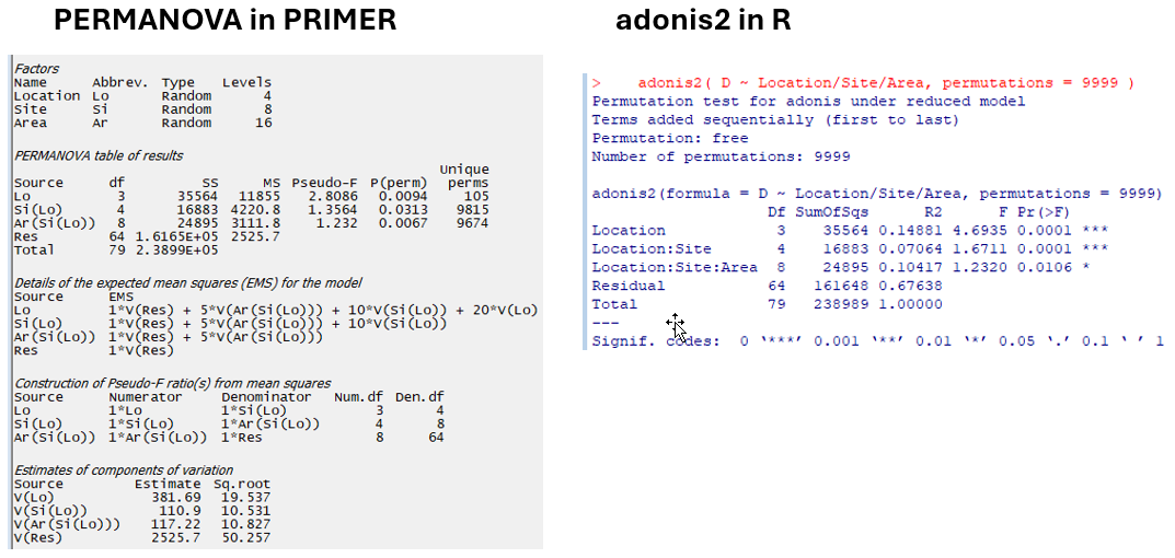 Fig. 1. Comparison of results for the holdfast data using PERMANOVA in PRIMER and adonis2 in R.
More specifically, although the degrees of freedom and the sums of squares are effectively identical (in this particular case), the pseudo-F statistics and the p-values are not (Fig. 2).
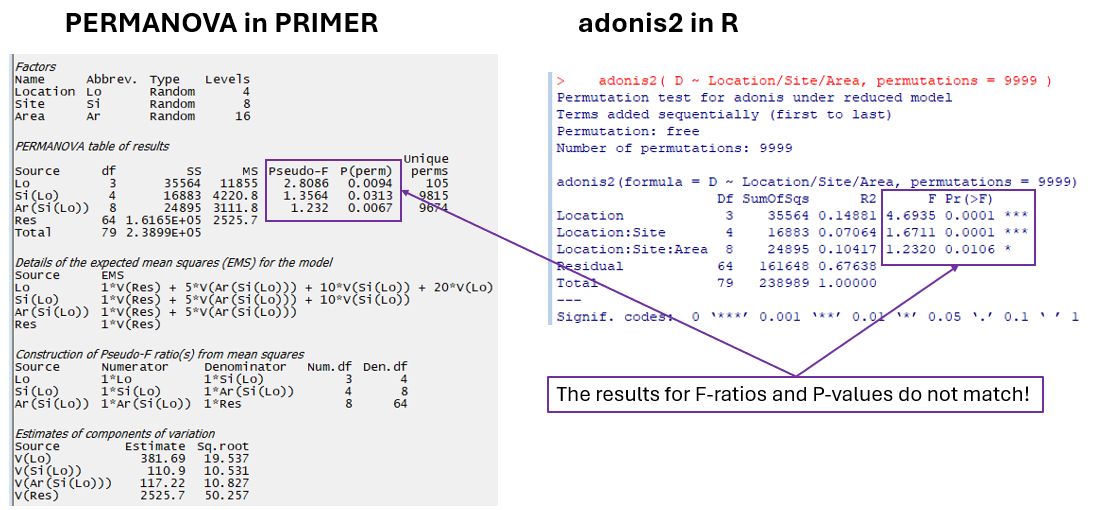
Fig. 2. Pseudo-F ratios and p-values do not match.
Why don't we get the same results as PERMANOVA in PRIMER when we run PERMANOVA using the adonis2 function in R? Unfortunately, the results obtained using adonis2 are incorrect. Basically, adonis2 takes no notice of whether factors are fixed or random. The adonis2 function gives you no way of specifying the types of factors you are dealing with; adonis2 treats all factors as if they are fixed. In contrast, PERMANOVA does the analysis correctly by reference to the full study design specified by the end-user.
3.3 How does PERMANOVA do it?
Following the PERMANOVA table of results, a suite of key additional details regarding the analysis can be seen in the PERMANOVA output file. These details highlight what makes the implementation of PERMANOVA in PRIMER so unique, surpassing all other software tools that we know of in its handling of multi-factorial sampling and experimental designs.
The implementation of PERMANOVA in PRIMER pays very careful attention to whether factors are fixed or random and whether they are crossed with or nested within other factors in the study design. The construction of correct test-statistics and permutation algorithms for every term in the model rely ciritically on the expectations of the mean squares.
Additional details in the PERMANOVA output file include (Fig. 3):
- details of the expected mean squares (EMS) for each term in the model;
- the construction of the pseudo-F ratios for each term in the model from the appropriate mean squares (along with the associated numerator and denominator degrees of freedom); and
- estimates of the components of variation for each term in the model in the space of the resemblance measure.
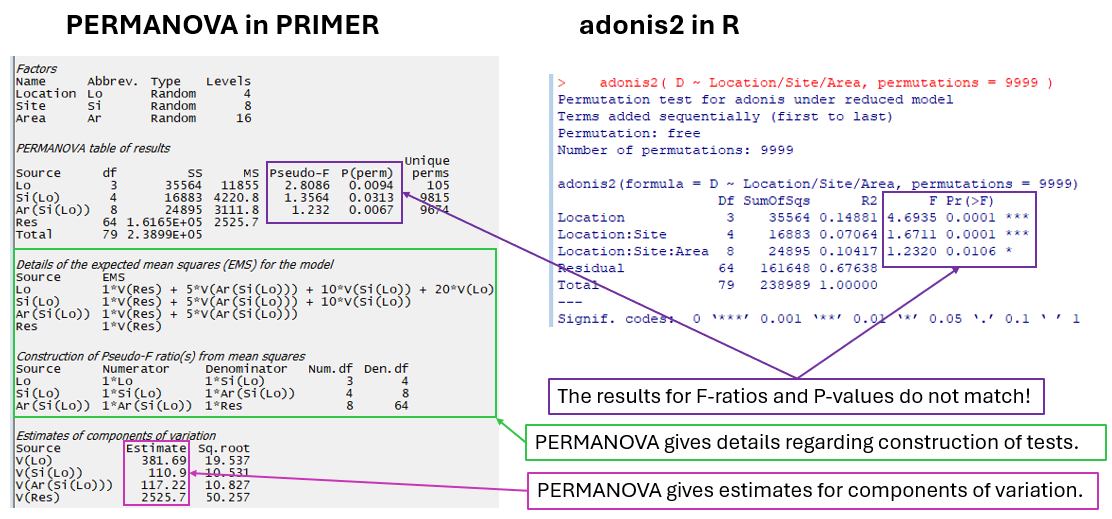 Fig. 3. Additional details provided in the output from a PERMANOVA analysis.
Expectations of mean squares
This portion of the output file shows which components of variation are involved (may contribute towards) the expectation of any given mean square (MS). For example, consider the mean square for the factor 'Location'. It is clear from the above output that variation among replicate holdfasts ('V(Res)'), Areas ('V(Ar(Si(Lo)))'), Sites ('V(Si(Lo))') and Locations ('V(Lo)') are all involved and hence can potentially contribute towards the expectation of the mean square (EMS) for Location.
Why do we bother with this? When we test individual terms in our model, it is absolutely vital that we build an F-ratio that focuses only on testing the null hypothesis associated with the term of interest. We must make sure not to confound its source of variation with other potential sources of variation inherent in our experimental design when we perform each individual test.
Construction of pseudo-F ratios
PERMANOVA in PRIMER uses the EMS information in order to contruct the correct pseudo-F ratio for the test of any individual component of variation (term) in any multi-factor model. This is done with careful consideration of fixed and random factors in mixed models and/or hierarchical (nested)-type study designs. For example, it is appropriate, in this three-factor nested study design, to construct the individual tests as follows:
| Source | Construction of pseudo-F statistic |
|---|---|
| Location | $F$$Lo$ = $MS$$Lo$ / $MS$$Si(Lo)$ |
| Site | $F$$Si(Lo)$ = $MS$$Si(Lo)$ / $MS$$Ar(Si(Lo))$ |
| Area | $F$$Ar(Si(Lo))$ = $MS$$Ar(Si(Lo))$ / $MS$$Res$ |
It would be incorrect, of course, to test 'Location' by placing $MS$$Lo$ directly over the residual mean square ($MS$$Res$) as the denominator. That approach will not account correctly for the other sources of variation (Areas and Sites) that may indeed contribute towards the mean square for 'Location'. This is true for multivariate dissimilarity-based analysis, just as it is for classical univariate ANOVA.
Permutable units
The denominator of the pseudo-F ratio also points us directly towards the correct permutable units for the test ( Anderson (2001b) ; Anderson & ter Braak (2003) ). By 'permutable units', we mean the items that should be considered 'exchangeable' under a true null hypothesis. Hence, if we are interested in testing the factor of 'Location', we must permute whole sites (there are 8 of them, and we need to keep the replicates within each site together as a unit) randomly across the 4 locations. It is not appropriate to permute replicate holdfasts just anywhere randomly across the entire study design for the test of 'Locations', just as it is not appropriate to use the residual mean square directly as the denominator for the test of 'Locations'.
The implementation of PERMANOVA in PRIMER always uses expected mean squares to get a correct rigorous test for every term in the model; specifically:
- to construct the correct pseudo-F ratio; and
- to implement a correct permutation algorithm, accounting for other terms in the model.
Permutation algorithm
P-values are obtained by PERMANOVA in PRIMER using permutation algorithms that are constructed specifically for each term in the model, after identifying:
- the correct permutable units (referencing the F-statistic's construction); and
- the correct reduced-model residuals, accounting for other terms in the model.
Using reduced-model residuals is the default in PERMANOVA. Alternatively, one can choose to permute raw data or full-model residuals, which are less optimal, but are fine asymptotically. Even so, this does not get away from the need to ascertain the correct permutable units, which is not really negotiable if you want to achieve the correct test for your study design.
Of course, each term will require its own denominator and its own permutation algorithm, which will depend on whether terms are fixed or random, whether there are nested terms, covariates or interactions, etc. For unbalanced cases, the 'Type' of sum of squares is also very important for the partitioning, the expectations, and subsequent tests.
Degrees of freedom
The additional information provided in the output also helps us to see where the degrees of freedom (df) from our full study design 'ended up' in the PERMANOVA analysis. From an experimental design point of view, it is important to try to maximise the denominator df, whenever possible, in order to obtain better power for tests of the term(s) of interest. For example, if we wanted to get more power to test for significant variability at the scale of Locations, then increasing the number of holdfasts per area would do little to help. We would be far better off increasing the number of sites sampled per location (even at the expense of reducing the number of holdfasts collected per area), precisely because the mean square for 'Site' is used as the denominator in the pseudo-F statistic constructed by PERMANOVA to test for variation among Locations.
Components of variation
Finally, the estimated components of variation are also extremely useful (provided at the bottom of the output file). These are calculated in a directly analogous way to univariate ANOVA estimators, relying (once again) on the expectations of the mean squares. The column labeled 'Estimate' is in squared dissimilarity units, and its square root ('Sq.root', interpretable as a sort of standard deviation in the space of the resemblance measure) is also provided.
In the present example, we can see that the greatest variation occurs at the smallest spatial scale - from holdfast to holdfast within a given area (i.e., the square root of 'V(Res)' is 50.257 in Jaccard % dissimilarity units). This means that holdfasts that are just a 'fin-kick' away (or so) from one another may share little more than half of their mollusc species! The sources of variation (in order of importance, as quantified by the PERMANOVA model) are: Residual > Location > Area > Site.
The values in the 'Estimate' column can be expressed (optionally) as percentages of the total (provided there are no negative estimates of variation in a given model), thusly:
| Source | Estimate (based on EMS) | Percentage |
|---|---|---|
| Location | 381.69 | 12.17 % |
| Site | 110.90 | 3.54 % |
| Area | 117.22 | 3.74 % |
| Residual | 2525.70 | 80.55 % |
| Total | 3135.51 | 100.00 % |
It is not uncommon in ecological field studies for the residual component of variation to be large relative to other sources of variation.
For more information about all of these key additional details provided in the PERMANOVA output file, please consult the PERMANOVA+ manual.
3.4 How does adonis2 do it?
The adonis2 function (in the vegan package in R) will provide a partitioning of the total sum of squares according to a given ANOVA design. However, adonis2 constructs pseudo-F ratios for all of the terms in any model using the residual mean square ($MS$$Res$) as the denominator (yikes!). In many cases, this will (clearly) give you incorrect results.
Thus, adonis2 has two fundamental drawbacks:
- It does not use expectations of mean squares to construct the correct F tests.
- It does not identify the correct permutable units for tests of individual terms in the model.
This means there are really important limits on what kinds of ANOVA models adonis2 can actually (safely) be used for. Specifically, adonis2 will not handle correctly any designs that have random factors or nested factors. It also may be problematic for cases where there are continuous covariates and/or imbalance in the study design, whenever these features affect the EMS (i.e., almost always).
In effect, adonis2 assumes everything is a fixed factor, and a sequential (Type I) SS is done. This function is therefore also quite limiting for analysing unbalanced ANOVA designs or designs with quantitative covariates. In contrast, PERMANOVA in PRIMER offers partitioning using Type I, Type II or Type III SS (your choice).
Are there cases when it might be ok to use adonis2?
An analysis done using adonis2 in R should be ok if you have a single factor (a simple one-way ANOVA design). It might be ok(?) if you happen to have all fixed factors in a fully balanced, fully crossed design, with no random factors, covariates or nested terms. (Caveat: I can make no promises about that)!
Clearly, as previously articulated in Chapter 2 above, R is a wonderful statistical programming language, with loads of packages that are constantly evolving, and with many amazing contributors, so maybe in the future the functionality of adonis2 will be improved, or a new package will be written. At the moment, however, you cannot trust R to analyse PERMANOVA models correctly except (perhaps?) in some very special cases (i.e., crossed fixed factors only, fully balanced designs).
In contrast, you can completely trust the implementation and resulting output provided by PERMANOVA in PRIMER for any design.
3.5 What about $R^2$ values?
Another clear difference between the output given by adonis2 by comparison with the output given by PERMANOVA in PRIMER is the fact that adonis2 provides an additional column, headed 'R2'. These are values of $R^2$ for a given term in the model, calculated directly as the ratio of an individual term's explained sum of squares (SSterm) divided by the total sum of squares (SStotal, Fig. 4). Unfortunately, the inclusion of this column is, in my view, misguided.
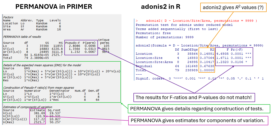 Fig. 4. PERMANOVA gives estimates for components of variation based on EMS, whereas 'adonis2' gives $R^2$ values in the output.
Why doesn't PERMANOVA output $R^2$ values?
Sums of squares (SS) are used to partition variation in the multivariate data cloud in the space of the resemblance measure according to each term in the PERMANOVA model. However, these SS values cannot be compared directly with one another, quite simply because they have different degrees of freedom (df). For example, the SS for a term with 64 df would automatically be expected to 'explain more' than a term with just 3 df. To put this quite simply in another way: a sum of squares is not the same thing as a variance.
In addition, the mean squares (MS) are also not able to be compared directly with one another. As already outlined above, the expectations of mean squares can (and very often do) include more than one source of variation, and this also must be taken into account when we wish to quantify the relative sizes and (hence) the relative importance of the effects (or terms) in any given model.
Values of $R^2$ can never be interpreted directly as 'effect sizes' in an ANOVA context. That is why we don't use raw $R^2$ values (the term's SS divided by the total SS) in order to quantify the relative importance of individual terms from a PERMANOVA (or ANOVA) model. This would be a mistake with the potential to mislead, even for a classical univariate ANOVA. (In contrast, it may be fine to use $R^2$ values in ordinary least-squares regression models for comparative purposes, considering one variable at a time, where every predictor variable is on an equal footing and has just 1 df.)
As it is potentially quite misleading to include $R^2$ values in an ANOVA table, PERMANOVA in PRIMER does not provide them in the output. Instead, it uses the EMS to carefully estimate components of variation for each term in the model. These components can indeed be directly compared to assess the relative importance/contribution of individual terms (sources of variation) in the model.
3.6 Summarising the comparison
In summary:
- I recommend using PERMANOVA in PRIMER.
- I do not recommend using adonis2 in R.
- Except in very limited circumstances, adonis2 does not construct:
- (i) correct F-ratios; or
- (ii) correct permutation algorithms.
- The implementation in adonis2 is far too limiting (it can only be correct for one-way cases, and possibly correct for fixed factors only in fully crossed, fully balanced designs).
- Furthermore, $R^2$ values for individual terms in ANOVA models are not a sensible way of comparing their relative importance.
It would be exhausting, fruitless and probably upsetting to list all of the papers that have used adonis2 (or adonis, its predecessor) in R to perform a PERMANOVA for a complex design that have failed to notice these important problems and limitations. No-one can really be blamed for trying to use adonis2. It seems (on the face of it) like it should work. It has been used to run all sorts of designs and gets cited rather a lot. Unfortunately, the results of analyses done using adonis2 might be wrong, and the inferences drawn misleading, depending on the model/study design.
In deference to the excellent people who wrote the adonis2 routine (it's clearly a good thing that they created it), I feel certain that they (probably) never intended for this function to be used to analyse complex experimental designs with random factors, nested factors, etc. It would be helpful for the truly limited scope of adonis2 to be more plainly acknowledged somewhere in the documentation and/or description of the routine, so that end-users are not mis-led. Perhaps a future R package will address some of these issues.
Importantly, the PERMANOVA routine in PRIMER allows the user:
- to specify whether factors are fixed or random,
- to specify whether a factor is nested in one or more other factors,
- to test interaction terms,
- to include one or more quantitative covariates in the analysis,
- to remove individual terms from a model or to perform pooling,
- to correctly analyse:
- fixed models, random models & mixed models
- user-specified contrasts
- BACI designs (before-after/control-impact),
- asymmetrical designs (e.g., in environmental impact studies),
- randomised blocks,
- split plots,
- hierarchical designs,
- repeated measures,
- unbalanced designs (Type I, II or III sums of squares),
- ... and more.
4. Take-home messages
4.1 Final cautionary notes
The purpose of this exposé has been to highlight some important pros and cons associated with using PRIMER and R in routine analytical work. It is clear that both R and PRIMER have great capabilities and using them both should be encouraged.
A genuine question about 'which one to use' really only arises when it is perceived that both PRIMER and R each have a specific routine that will (purportedly) do the same thing. For example, both adonis2 (in the vegan package) in R and PERMANOVA for PRIMER assert the ability to implement a dissimilarity-based permutational multivariate analysis of variance. At the current time, PERMANOVA in PRIMER has a far greater scope and capacity than adonis2 to achieve this, and (unlike adonis2) its results are correct and reliable for any design.
In Chapter 3 above, we compared the results of a PERMANOVA obtained using PRIMER vs R for a specific dataset. We showed that using an R routine outside its limits is a dangerous and flawed enterprise. It turns out there are a lot of other routines in R like the adonis2 function in this respect: they allegedly perform a certain analysis, but may in fact have an inherent weakness in their design, or limitations that are not obvious from a casual (or even a detailed) glance at the available documentation. It becomes clear upon inspection that a broad range of specialised methods available in PRIMER (such as PERMANOVA, PERMDISP, CAP, multi-way ANOSIM, BEST, etc.) are not able to be replicated using any available R packages at the present time.
A lot of R packages (or freely available R code) may look, on the face of it, to be able to do an analysis you want to do. Please bear in mind that there may be:
- problematic assumptions that can lead (unexpectedly) to incorrect results; or
- important limitations (not necessarily obvious) on their correct use.
When using a given R routine, here are some questions you should probably ask yourself:
- How will you know if the results are reliable?
- Can you check it by programming it independently yourself?
- What will it do for your particular use-case at this particular time?
- Are you prepared to re-check a given R routine again when you use it at a different time and for every new use-case you wish to throw at it?
4.2 Should I use PRIMER or R? (in short)
Use Both!
The take-home message here is: use both! Neither replaces the other. They are good at different things.
- R is a wonderful programming language and is very flexible and general. You can use it to do heaps of stuff, but it is difficult to use well. Depending on the package, you cannot always trust it without doing a lot of additional checks. It is easy to make mistakes - you need to debug your code and make sure you use existing packages within their scope. Correct functioning may depend on context and can also vary over time.
- PRIMER is an excellent software package with a narrower focus. What it does, it does exceptionally well. It specialises in performing a suite of robust multivariate methods, many of which are simply not available in R (or any other software). It is very easy to use and you can trust the results.
When do I use what?
In my own work, I use PRIMER first and foremost for all the stuff that it can do and is really good at, not just because it is easier (which is reason enough), but also because I know I can trust the results. I use R for most other things, and with few exceptions I program and de-bug my own R code. Breaking this down into some concrete recommendations:
Use PRIMER (with PERMANOVA+) for:
- Robust dissimilarity-based multivariate analysis in general
- Non-parametric methods
- ANOSIM, BEST, RELATE, MDS, CLUSTER, ... etc.
- Semi-parametric methods
- PERMANOVA, PERMDISP, DISTLM, dbRDA, CAP, ... etc.
- other methods unique to PRIMER (or better-implemented or easier to run in PRIMER)
- Second-stage MDS, threshold-metric MDS, BVSTEP, LINKTREE, SIMPROF, custom-ordered shade plots, segmented bubble plots, biodiversity metrics, taxonomic distinctness, functional resemblance, ... etc.
Use R for:
- Running routine classical stats
- Programming bespoke data wrangling
- Tailoring graphics
- Creating and testing new statistical ideas or methods
- Running a specific analysis/method using a package that you know, trust and have checked thoroughly for your particular application or context.
- Running simulations, etc.
I sincerely hope that this contribution will help researchers get the most from their software tools for data analysis. The focus of this exposé has been exclusively on PRIMER and R, as the specific question 'Should I use PRIMER or R?' seems to keep bubbling up. There are clearly a large number of other statistical software options out there (with their own pros and cons) and I would encourage researchers to explore them as well, with an open mind.