1. Expanded summary statistics

• 1.1 Expansion from P7 to P8
• 1.2 Definitions of statistics
• 1.3 Biotic data: summary stats
• 1.4 Split summary stats results by groups
• 1.5 Environmental data: summary stats

1.1 Expansion from P7 to P8

Summary statistics provide essential information to help you get to know your variables, their fundamental statistical properties and numerical characteristics. In P8, if you click on Tools > Summary Stats... you will see (Fig. 1.1) that we have greatly expanded the list of options on offer, compared to those available in P7 (where it used to be accessed under Analyse > Summary Stats...). In some cases, you may wish to calculate summary statistics across the values you are getting across a sample, so this is catered to as well (just as in P7). We have also added the possiblity to output summary statistics separately for different levels of a factor (or different groups of an indicator, in the event that you are summarising samples instead of variables).

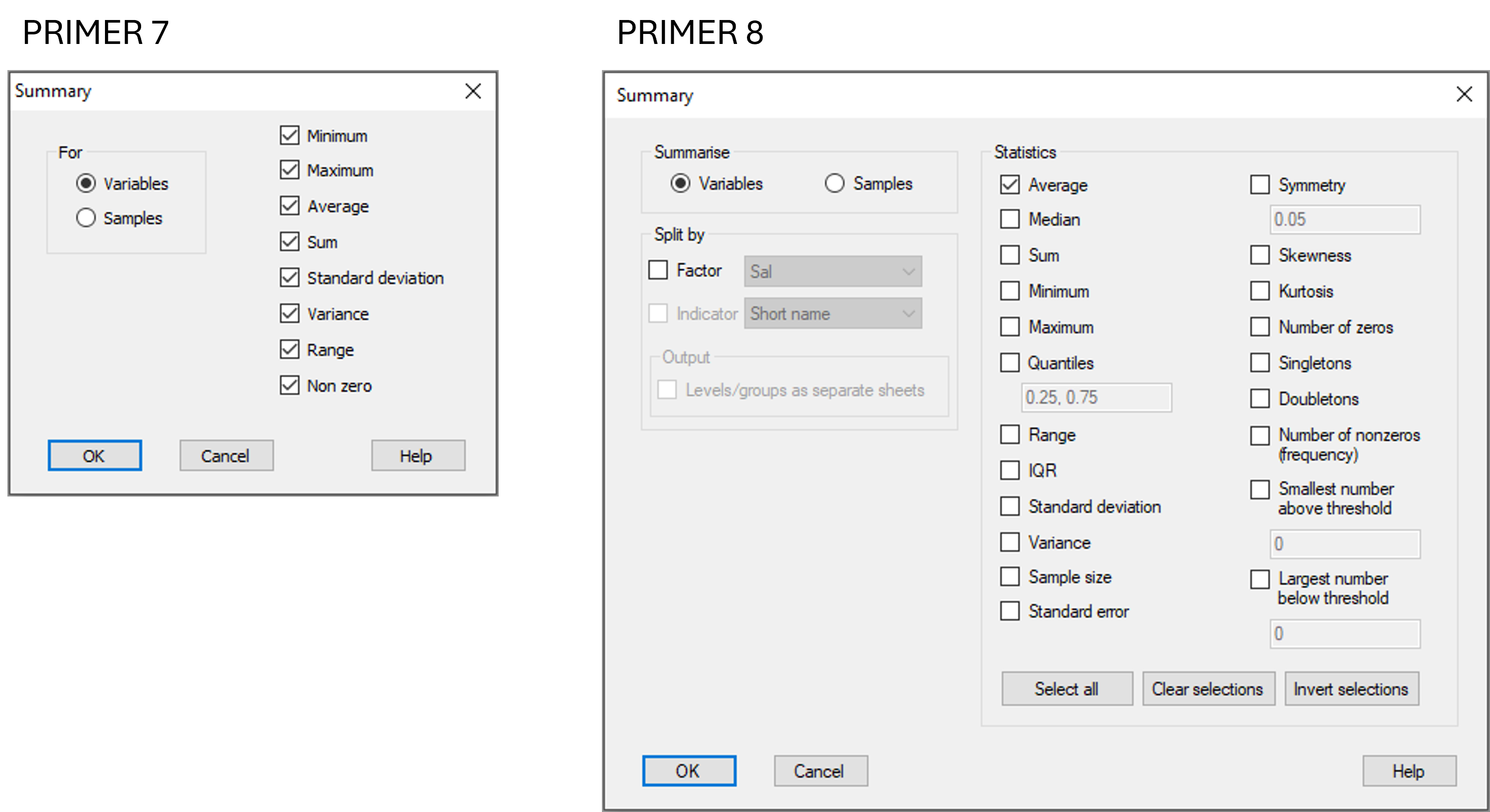
Fig. 1.1. Comparison of the 'Summary Stats...' dialog options in PRIMER 7 vs PRIMER 8.

In what follows, we shall begin by providing a brief description of each of the summary statistics, then demonstrate the use of this new tool by implementing it to summarise information about variables (i.e., across samples). Note that you can also use this tool to summarise information about samples (i.e., across variables).

1.2 Definitions of statistics

Given a set of values $\{ y_1, y_2, ..., y_n \}$ for any individual variable $Y$, the following summary statistics can be calculated by clicking on Tools > Summary Stats... in PRIMER 8:

• Average: $\hspace{1mm}$ $\bar{y} = \sum_{i=1}^n{y_i} / n $, the average (or mean)
• Median: $\hspace{1mm}$ $m$, the median value
• Sum: $\hspace{1mm}$ $\sum_{i=1}^n{y_i}$, the sum of the values
• Minimum: $\hspace{1mm}$ $\min(y_i)$, the minimum value
• Maximum: $\hspace{1mm}$ $\max(y_i)$, the maximum value
• Quantiles: $\hspace{1mm}$ $q_\alpha$, the value corresponding to a given ($\alpha$-)quantile in the empirical distribution of values. Quantiles must be chosen by the end-user and must be in the range (0, 1).
• Range: $\hspace{1mm}$ the range; i.e., $(\max(y_i) - \min(y_i))$, the difference between the maximum and minimum values
• IQR: $\hspace{1mm}$ the inter-quartile range; i.e., $(q_{0.75} - q_{0.25})$, the difference between the upper and lower quartile.
• Standard deviation: $\hspace{1mm}$ $s$, the standard deviation; i.e., the square root of the variance.
• Variance: $\hspace{1mm}$ $s^2=\sum_{i=1}^n{(y_i - \bar{y})^2} / (n-1)$, an unbiased estimate of the variance.
• Sample size: $\hspace{1mm}$ $n$, the number of values
• Standard error: $\hspace{1mm}$ $\sqrt{s^2/n}$, the standard error of the mean
• Symmetry: $\hspace{1mm}$ $\alpha$-symmetry statistic, with $\alpha$ chosen by the end-user (default $\alpha$ = 0.05). For symmetric data, the median ($m$) is equidistant from the $\alpha$-quantile and the $(1-\alpha)$-quantile. The $\alpha$-symmetry statistic is defined as $(m-q_{\alpha}) / (q_{1-\alpha} - q_{\alpha})$ for a given quantile ($\alpha$). A value close to 0.5 indicates symmetry, a value < 0.5 indicates right-skewness, and a value > 0.5 indicates left-skewness.
• Skewness: $\hspace{1mm}$ $k_3$, the skewness coefficient; i.e., $$ k_3 = \frac{ n \sum_{i=1}^n (y_i - \bar{y})^3 } { (n-1)(n-2) \cdot s^3 } $$A value close to zero indicate symmetry. A positive value indicates right-skewness; a negative value indicates left-skewness. See Sheskin (2011) .
• Kurtosis: $\hspace{1mm}$ $k_4$, the kurtosis coefficient; i.e., $$ k_4 = \frac{ \left[ \left[ \sum_{i=1}^n (y_i - \bar{y})^4 (n)(n+1) \right] / (n-1) \right] - 3 \left[ \sum_{i=1}^n (y_i - \bar{y})^2 \right]^2 } { (n-2)(n-3) \cdot s^4 } $$ A value close to zero indicates a mesokurtic distribution. A positive value indicates a leptokurtic distribution (pointy, with broad tails). A negative value indicates a platykurtic distribution (flat-topped, with short tails). See Sheskin (2011) .
• Number of zeros: $\hspace{1mm}$ the number of zeros.
• Singletons: $\hspace{1mm}$ the number of ones (useful for count data).
• Doubletons: $\hspace{1mm}$ the number of twos (useful for count data).
• Number of nonzeros (frequency): $\hspace{1mm}$ the number of non-zero values; e.g., if the variable consisted of counts of an organism, this would be the frequency of occurrences of that organism across the set of values (samples).
• Smallest number above threshold: $\hspace{1mm}$ the smallest value in the set that occurs above a specified threshold value ($y_t$), chosen by the end-user. For example, to obtain the smallest non-zero value in a set of non-negative values, specify $y_t=0$. Here is another example: suppose a variable consists of lead (Pb) concentrations measured from sediment. It may be useful to identify the smallest concentration value recorded above the detection limit of the instrument. Knowing the smallest non-zero (or detected) value can be handy for choosing an appropriate constant ($c$) to add for a transformation such as $log(y+c)$, when the variable contains zero values.
• Largest number below threshold: $\hspace{1mm}$ the largest value in the set that occurs below a specified threshold value ($y_t$), chosen by the end-user. This option has similar uses to the previous one, but for non-positive data.

1.3 Biotic data: summary stats

To show the utility of this tool, we will calculate some summary statistics from a study examining changes in macrofaunal communities inhabiting sediments near an oil platform (Ekofisk) in the North Sea, provided by Gray et al. (1990) . These data consist of counts of the abundances of $p$ = 174 taxa (mostly identified to species level) sampled by 3 day grabs taken at each of $N$ = 39 stations, situated in an approximately 5-spoke radial design leading out from the oil platform. The stations were classified into the following four groups according to their relative distance from the centre of drilling activity at the Ekofisk oil platform: D = less than 250m, C = 250m - 1km, B = 1 - 3.5km, and A = more than 3.5km away.

Start running PRIMER 8, then click File > Open... to open the data file named 'Ekofisk_macrofauna_counts.pri' (found inside the 'Examples_P8 > Ekofisk_macrofauna' folder).

From the 'Ekofisk_macrofauna_counts' data sheet inside PRIMER, click on Tools > Summary Stats..., as shown below:

Choose from the dialog all of the summary statistics you would like to calculate on the dataset. For example, we might choose to calculate the average, median, minimum, maximum, range, standard deviation, number of zeros, singletons, and the number of non-zeros (i.e., frequency of occurrence), like this:

Click 'OK', and you will see a 'Summary Statistics 1' file, in which you are shown the choices you made for running that routine, viz:

as well as a resulting output file 'Data1', which provides all of these summary statistics for each of the individual variables (taxa), as shown below:

1.4 Split summary stats results by groups

To run summary statistics on your variables separately for multiple groups of data, just choose a factor by which you would like to split the data in the dialog. For example, for the Ekofisk dataset, suppose we wished to obtain summary statistics (means and standard errors) separately for each of the 'Distance' groups. We can achieve this by choosing Tools > Summary Stats... > (Summarise > $\bullet$Variables) & (Split by > $\checkmark$Factor > Dist) & (Statistics > $\checkmark$Average & $\checkmark$Standard Error), as shown in the dialog below:

By default, PRIMER will provide the output for each summary statistic you have asked for as a separate data sheet, and the groups (corresponding to levels of the factor by which you have chosen to do the splitting), will be the 'Samples'. In the present example, you will see that the averages for each variable for the four distance groups (A, B, C, D) have been provided in 'Data2' and the standard errors are given in 'Data3'. There will be as many new data sheets generated as there are summary statistics asked for in the dialog. Note that the name of the summary statistic provided in each sheet is given in the title at the top of the sheet, e.g., 'Ekofisk oilfield macrofauna -Summary Statistics, Average'.

An alternative output format can be requested here, with results for different groups given on different sheets. To do this, choose Tools > Summary Stats... > (Summarise > $\bullet$Variables) & (Split by > ($\checkmark$Factor > Dist) & (Output > $\checkmark$Levels/groups as separate sheets)) in the dialog, like so:

Doing this yields a separate sheet of summary statistics for each of the groups (e.g., 'Data4' has all of the summary statistics you requested calculated for group D only, 'Data5' has the results for group C, and so on (see below). Note that, for this alternative type of output, the name of the factor on which the split was done and the specific group (factor level) is given in the title at the top of each new data sheet of results; for example, 'Ekofisk oilfield macrofauna -Summary Statistics, Dist: A'.

1.5 Environmental data: summary stats

For environmental data, we might choose to calculate different sorts of summary statistics than the kinds of things we would want to know about biotic data consisting of counts. For count data, quantities like the numbers of zeros, singletons, doubletons and frequencies of occurrence might well be of interest. However, these are not typically meaningful for variables that have been recorded as (effectively) continuous values, such as temperature, dissolved oxygen, etc. Instead, when we deal with environmental data (or, more generally, continuous quantitative variables), it may be helpful to know what the smallest non-zero value is, or to know the degree of skewness. These can aid in determining an appropriate transformation (e.g., to obtain approximate symmetry).

Let's look at some environmental data from a study of benthic soft-sediment assemblages in the Firth of Clyde, SW Scotland ( Pearson & Blackstock (1984) ). The abundance and biomass of 84 macrofaunal species as well as contaminant data (organic enrichment and concentrations of heavy metals in the sediment) were sampled at a series of 12 sites along a transect that passed through the sewage-sludge disposal ground at Garroch Head. Open the data file named 'Clyde_environment.pri' in PRIMER (found inside the 'Examples_P8 > Clyde_macrofauna' folder).

Of course, tools such as histograms and draftsman plots (found under the Plots menu) are very useful for visualising the distributions of values for the individual variables. Summary statistics complement these visual tools, yielding some important additional detailed information. Click Tools > Summary Stats..., then choose to output the following statistics (shown in the dialog below): average, minimum, maximum, standard deviation, symmetry (0.05), skewness, kurtosis, and smallest number above a threshold of 0.

The resulting output file (called 'Data1' and shown below) indicates that many of the variables are right-skewed, with positive values for skewness, and values less than 0.5 for the symmetry statistic, while others (Co, Ni) are apparently left-skewed (negative skewness and symmetry > 0.5). Depth, however (Dep) is a fairly flat (platykurtic) variable (with negative excess kurtosis). Also evident is the fact that values of cadmium concentration (Cd) reach a minimum value of zero, and that the smallest value recorded above zero is 0.1. Thus, if we were inclined to transform the values for Cd (e.g., to make its distribution more symmetric), we might consider a log transformation such as $log(y_i+c)$, where $c$ = 0.1.

(Note: the variable 'Cd' has been highlighted in the above image of 'Data1' by clicking on the heading for that column. Highlighting variables (or samples), can be very useful for selecting subsets of data, or for applying a transformation to a subset of variables.)