11. Residual distances

11.1 What are 'residual' distances?
11.2 Example: Plankton (revisited)

11.1 What are 'residual' distances?

Rationale

It is sometimes desirable to remove the effects of a factor or covariable, and examine 'what is left', i.e., to look at variation in residuals. For example, a factor of primary interest may be statistically significant in a PERMANOVA partitioning of the full model, but its effects may be totally obscured by some other dominant factor(s) or covariate(s) when we look at an ordination of the data.

As seen in Chapter 10, we can construct plots of distances among centroids for main effects and interactions, and these kinds of plots may shed some light on the nature of some minor effects in any given model. Another tool that can help us see effects occurring along minor axes that may not be apparent in unconstrained plots is canonical analysis of principal coordinates (CAP). Nevertheless, a dissimilarity-based multivariate analogue to a residual plot, from which the variation due to dominant (but perhaps nuisance) factors or covariates has been removed, is desirable ( Anderson (2017) ).

Construction of residual dissimilarities

Our description here paraphrases Anderson (2017) . Suppose we have a symmetric matrix, ${\bf D}$, of dissimilarities among sampling units, having elements $\lbrace d_{ij} \rbrace$, $i = 1, \ldots, N$ and $j = 1, \ldots, N$. We have seen earlier how to derive Gower's matrix, ${\bf G}$ from this (see Gower (1966) ), which is also of size $(N \times N)$ and is comprised of elements $\lbrace g_{ij} \rbrace$. The trace (sum of diagonal elements) of matrix ${\bf G}$ is equal to the total sum of squares (total variation) in the space of the chosen dissimilarity measure.^¶

Let's now suppose that ${\bf X}_ r$ is a linear model matrix which contains one or more covariables and/or orthogonal contrasts for one or more factors that we wish to 'remove'. By 'remove', we mean 'on which to condition'. For example, suppose we have a two-factor study design, with factors A and B, and we wish to 'remove' the effects of factor A (e.g., to investigate and hopefully visualise in ordination plots, etc., the effects, if any, of factor B). This amounts to 'taking factor A into account' in our examination of factor B. In such a case, matrix ${\bf X}_ r$ will be a full-rank matrix of orthogonal contrasts among the groups in factor A. Now, for any model matrix ${\bf X}_ r$, we can construct the usual linear projection ("hat") matrix as:

$$ {\bf H}_ r = {\bf X}_ r [ {\bf X}_ r'{\bf X}_ r ]^{-1} {\bf X}_ r' $$

We then obtain a 'residualised' Gower matrix directly as

$$ {\bf G}^{[R]} = ({\bf I} - {\bf H}_ r) {\bf G} ({\bf I} - {\bf H}_ r) $$

where ${\bf G}^{[R]}$ is an $(N \times N)$ matrix with elements $\lbrace g_{ij}^{[R]} \rbrace$. We note, in passing that $\text{tr}({\bf G}^{[R]})$ is the residual sum of squares after fitting the full model contained in matrix ${\bf X}_ r$. Once we have this residualised Gower matrix, it is a straightforward back-transformation to arrive at an $(N \times N)$ matrix of residual distances, ${\bf D}^{[R]}$, with elements:

$$ \lbrace d_{ij}^{[R]} \rbrace = \sqrt{ g_{ii}^{[R]} - 2g_{ij}^{[R]} + g_{jj}^{[R]} } $$

This residualised distance matrix, ${\bf D}^{[R]}$, can then be examined in the usual way via ordination methods, such as mMDS, tmMDS or nMDS. The effects of any factors included in ${\bf X}_ r$ (and/or, the linear relationships in the resemblance space with any covariables in ${\bf X}_ r$) will be 'removed' from the picture.

The concept of removing a factor

In essence, the removal of a factor is equivalent, conceptually, to superimposing the group centroids onto a common (overall) centroid. For example, let's re-visit the 2-factor crossed study design by Glasby (1999) . In this study, the cover of subtidal epifauna was quantified on subtidal settlement plates in response to two crossed factors: Position ('N' = near the seafloor, 'F' = far from the seafloor) and Shade ('S' = shaded, 'C' = procedural control, 'O' = open).

A non-metric MDS plot of these assemblages on the basis of the Bray-Curtis resemblance measure, after a square-root transformation of the raw cover values, is shown in Fig. 11.1 below (this plot is a replica of Fig. 10.2 above).

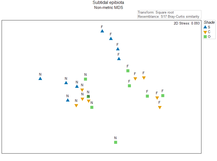
Fig. 11.1. Non-metric MDS of the individual sampling units from the two-factor crossed study design described by Glasby (1999) . Symbols correspond to the factor of 'Shade' ('S' = Shade, 'C' = Procedural Control, 'O' = Open surfaces), and labels correspond to the factor of 'Position' ('N' = Near, 'F' = Far).

The most obvious structuring factor here is Position; there is a large gap between samples that are near ('N') vs far ('F') from the seafloor. Let's suppose that we want to see more clearly the effects of Shade, and so we want to get residual distances after removing^† the (larger) effect of Position.

Let's use the 2D Euclidean distances in the nMDS plot as a proxy for the full Bray-Curtis space here, just to help visualise what happens when we 'remove' effects. The effects of the Position factor (as represented in the 2D nMDS plot) are shown in Fig. 11.2 below. These are simply the deviations of the individual group centroids ('N' and 'F') from the overall centroid.

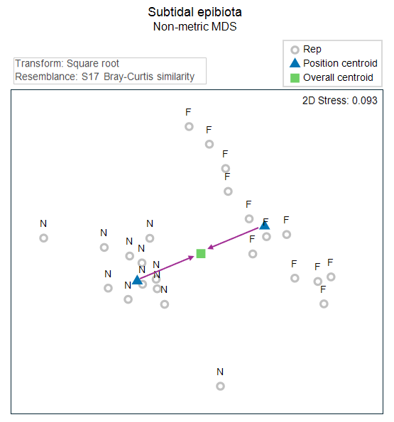
Fig. 11.2. Non-metric MDS precisely as in Fig. 11.1, but here showing only the labels correspond to the factor of 'Position' ('N' = Near, 'F' = Far), along with the centroids for each group (in blue), the overall centroid (in green) and the effects (arrows in a plum colour).

Now, to remove these effects, the steps are as follows:

(i) Estimate the centroids for each 'Position' group (near and far); these will be calculated as the average of all of the samples along each of nMDS axis 1 and nMDS axis 2, done separately for each group.
(ii) For each sample within a given group, subtract off the average for that group from its value (score) along nMDS axis 1, and do the same along nMDS axis 2; this operation removes the effect of 'Position' so that both the near and far samples are centered on a common (overall) centroid.
(iii) Replot the samples anew after this centering operation.

This action of centering the groups onto a common centroid (i.e., of removing the effects of Position), done in the 2d nMDS space, is shown in Fig. 11.3 below.

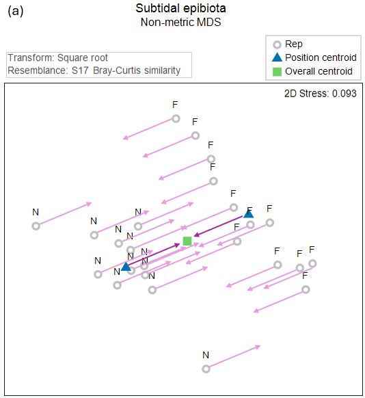
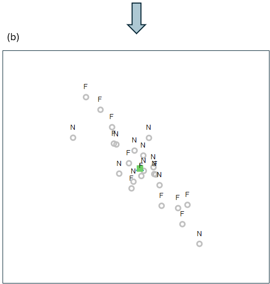
Fig. 11.3. (a) Non-metric MDS precisely as in Fig. 11.2, but here showing also the action of removing the Position effects from each sample unit (arrows in a light plum colour); and (b) the 'residual' plot of all the samples after removing the Position effect in this 2d nMDS space.

If we now put symbols corresponding to the factor of 'Shade', we can see the separation of assemblages in the Shade treatment from those in the Open and Control assemblages very clearly, and without any 'interference' from the effects of 'Position' in our plot (Fig. 11.4).

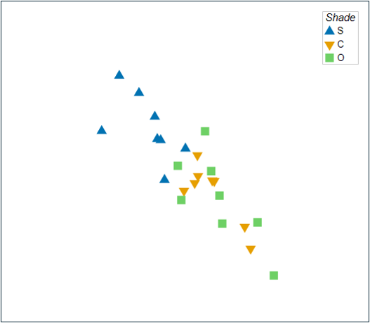
Fig. 11.4. The 'residual' plot of all the samples after removing the Position effect in this 2d nMDS space, precisely as in Fig. 11.3(b), but here showing symbols for the factor of Shade.

The above is a useful exercise to see how the effects of a factor can be removed in a 2D Euclidean nMDS space (Figs. 11.2 - 11.4). However, what we really want here is to perform this 'removing' operation in the full high-dimensional space of the chosen resemblance measure, hence to obtain a residual distance matrix, which then can be plotted via ordination.

Obtain a residual distance matrix and residual ordination plot

A residual distance matrix can be obtained after removing the effects of factors (and/or covariates) that have been specified in a given PERMANOVA design file by running the PERMANOVA+ > PERMANOVA... routine in PRIMER 8 and choosing (under the word 'Action' in the dialog) '$\bullet$Output residual distance matrix', as shown below.

The samples in that residual distance matrix, once created, can then be plotted via an ordination method of choice (typically nMDS) in the usual way.

Thus, for the data from Glasby (1999) , if we obtain a residual distance matrix in this way from a PERMANOVA design file with one factor ('Position'), then run nMDS on those residual distances, the resulting residual ordination plot looks like this (Fig. 11.5):

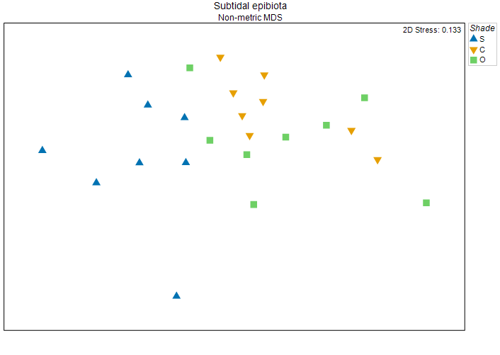
Fig. 11.5. Non-metric MDS plot of a residual distance matrix obtained after removing the effects of the factor 'Position' in the full-dimensional Bray-Curtis space. Symbols correspond to the factor of 'Shade' ('S' = Shade, 'C' = Procedural Control, 'O' = Open surfaces).

This plot shows (with a tolerable level of stress) the inter-sample relationships among multivariate residuals, after removing 'Position' effects in the high-dimensional Bray-Curtis space. The effects of shading on these subtidal epibiotic assemblages are very clearly seen now, indeed.

Removing quantitative (co)variables

It is possible to 'residualise' a distance matrix for a model that contains one or more quantitative covariables, even in the absence of any factors. This is done by fitting specified predictor variables (that is, the covariables you want to remove) in PERMANOVA+ > DistLM..., and ticking the box '$\checkmark$Output residual distance matrix' in the DISTLM dialog (e.g., see below).

In this case, it is the linear relationships between the covariable(s) and the distribution of samples in the high-dimensional resemblance space that are 'removed'; of course, non-linear relationships (if any) may remain. The samples in that residual distance matrix can then of course be plotted via an ordination method of choice (typically nMDS) in the usual way.

Stress in residual ordination plots

In the example above, we see that the stress of the residual nMDS plot (Fig. 11.5, stress = 0.133) is a bit larger than the stress of the original nMDS configuration (Fig. 11.1, stress = 0.093). This is somewhat to be expected. If there are major structuring forces creating patterns in a multivariate data cloud, like strong effects of a particular factor that 'pulls' sets of samples (e.g., from different groups) away from each other, then the stress will tend to be relatively low, compared to an unstructured (but otherwise similar) multivariate data cloud (i.e., that looks like a 'ball of fuzz'). Consider: it is rather easy to show a clear difference between (say) two groups of samples in 2 dimensions when the rank order relationships among samples are the main (only) thing we are trying to maintain (as in an nMDS).^‡ In contrast, a lack of structuring forces effectively makes it harder to push high-dimensional information into small (2D or 3D) spaces. Thus, when we 'remove' some (one or more) primary factors that do create structure in any particular study and look at 'what is left' in a residual ordination plot, we may well be met with relatively high stress. This is a generalisation, and may not always be the case. It may well depend on how much additional structure (e.g., due to other, more minor factors), still remains. In the example above the difference in stress is fairly modest and poses no difficulties for interpretation.

A note of caution regarding tests of significance

In most cases, a residual distance matrix should not be used as input into secondary routines in order to test hypotheses regarding the significance of a factor (or variable) after 'removing' some other terms specified in ${\bf X}_ r$. The reason for this is that the testing procedures in PRIMER/PERMANOVA+ use permutation methods to obtain p-values. Interestingly, even though you think you have 'removed' the effects of a nuisance factor (say), and so it seems you have already correctly 'conditioned' upon it, it turns out that this 'conditioning' is not maintained once you then go and permute the data. Essentially, when you have a residual distance matrix, its behaviour under permutation is no longer guaranteed to be independent of the thing(s) you thought you had removed.

Fortunately, when you do a multi-factor PERMANOVA with all terms in the model (including nuisance factors, or anything else you'd like to 'remove'or 'account for'), the conditioning on terms that are not being tested is perfectly maintained for every individual test that is done (i.e., for each line of the PERMANOVA output table). The nature of the conditioning done does depend on the Type of sum of squares, but this choice is fully under the control of the end-user and, once chosen, is perfectly maintained throughout all of the tests. Similarly, when you do sequential tests in DISTLM, the conditioning (on all previously fitted terms) is maintained perfectly, including under permutation. The essential trick here is to re-residualise for the terms you are trying to condition upon after every permutation. For more details, see Anderson & Legendre (1999) and Anderson & Robinson (2001) .

Suffice it to say that, generally, it is not wise to run tests on residual distance matrices, but they can be very useful tools for visualising patterns that might be difficult to see in typical ('unconditioned' and 'unconstrained') ordination plots.

^¶The value of $\text{tr}({\bf G})$ is also equal to the total sum of squared inter-point dissimilarities in ${\bf D}$ divided by the number of sampling units, $N$.

^†When we say 'removing' the effects, we could also say 'conditioning on' or 'accounting for' those effects.

^‡The most extreme example of this situation is reflected by the zero stress that is obtained as a 'degenerate solution', and a 'collapsed' nMDS occurs. For example, see section 5.2 in Change in Marine Communities.

11.2 Example: Plankton (revisited)

We shall show the utility of being able to construct a residual distance matrix and, from this, a residual ordination plot, by reference to a study of differential catches in plankton nets by Winsor & Clarke (1940) , provided by Snedecor (1946) . We met this dataset earlier, as an example of the use of the Wilcoxon signed-rank test. Recall that these data consist of the total log abundance values for each of five different types of plankton (hence, five variables, named using Roman numerals I, II, III, IV and V) that were caught in each of 2 nets towed simultaneously at 2 different depths: one at 29 m and the other at 31 m. There were ten hauls done in this way. The factors associated with these data are:

Position (either the upper (U) or the lower (L) net: a fixed factor); and
Haul (10 hauls labeled 1-10: a random factor).

Earlier (in the context of the Wilcoxon signed-rank test) we considered only a single variable - the total sum of the log abundances across all plankton types. Here, however, we are interested in examining the full multivariate dataset with all original $p$ = 5 variables. These data are located in the file ‘Woods_Hole_zooplankton.pri’, found inside the 'Examples_P8 > Woods_Hole_zooplankton' folder.

Visualise the main patterns using ordination

Open up the file (‘Woods_Hole_zooplankton.pri’) in PRIMER. The data values provided here are already expressed as log abundance values, so there is no need to apply any transformation.

From the 'Woods_Hole_zooplankton' data sheet, calculate a Bray-Curtis resemblance matrix by clicking Analyse > Resemblance and taking all the defaults (click 'OK'). The result will be 'Resem1', as shown below:

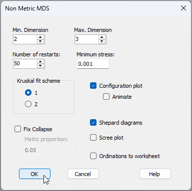
Next, create a non-metric MDS plot to visualise the patterns of inter-sample relationships among the plankton communities caught in these nets, based on the Bray-Curtis resemblances. From 'Resem1', click Analyse > MDS > Nonmetric MDS (nMDS).... Accept all of the defaults in the 'Non Metric MDS' dialog and just click 'OK'.

When you get the multi-plot output, you will see that 'Graph1' in the Explorer tree has the lowest-stress 2D nMDS plot achieved by the routine. From 'Graph1', click Graph > Sample Labels & Symbols... and choose the Labels to be plotted according to the factor of 'Haul', and the Symbols to be plotted according to the factor of 'Position', like so:

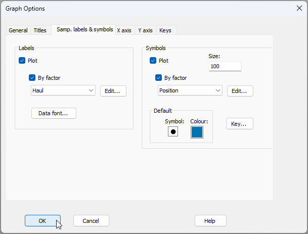
The resulting nMDS plot looks like this:

In the above ordination, there do not appear to be any obvious effects on these plankton communities attributable to the factor of 'Position'. Specifically, the symbols corresponding to assemblages caught in Upper ('U') vs Lower ('L') nets are scattered throughout the plot and look to be well mixed throughout this 2D MDS space. If anything, individual 'Hauls' seem to be more important in explaining variation here; we can see assemblages associatd with specific hauls (i.e., the two matching numbers, such as the two 7's, the two 3's, the two 8's, etc.) are often fairly close to one another in this nMDS plot.

However, it is possible that differences between the assemblages from one haul to the next are masking genuine differences due to Position, which may be smaller in size and/or may occur in a different direction than is captured by the nMDS ordination plot of reduced dimension. Of course, we should rely upon a two-way PERMANOVA (or ANOSIM)^‡ to formally test for significant effects in either of these factors.^¶

Run a two-way PERMANOVA analysis

Create a design file in accordance with the desired two-factor PERMANOVA model. From 'Resem1', click PERMANOVA+ > Create PERMANOVA Design.... In the resulting design file, called 'Design1', add a row (so there are 2 rows in total), then click inside the appropriate cells in the first column to choose the two factors: 'Haul' and 'Position' in rows 1 and 2, respectively. Also specify the factor of 'Haul' as 'Random' (under 'Type' in column 3), while 'Position' will remain as 'Fixed'. The resulting design file should look like this:

Now run the PERMANOVA analysis on the basis of this design. From 'Resem1', click PERMANOVA+ > PERMANOVA, then click 'OK' to take all the defaults here (the 'Design worksheet' should default to 'Design1' and all else is fine).

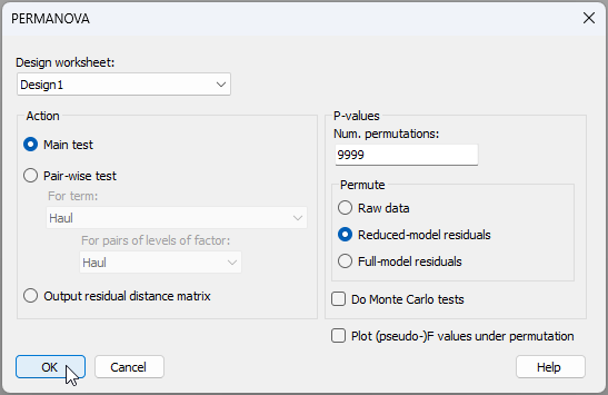
The key results in the output file (called 'PERMANOVA1' in the Explorer tree) look like this:

There is significant variation in these plankton assemblages from haul to haul ($F_{9,9}$ = 6.6, $P$ < 0.001). There is also a significant effect caused by the position (relative depth) of the nets ($F_{1,9}$ = 5.9, $P$ < 0.05). The effect size for the factor of 'Position' was much smaller than that for 'Haul' (see the relative sizes of these in the table labeled 'Estimates of components of variation' in the above output). We can therefore conclude that, in the initial nMDS plot, the significant effects due to the position of the nets are effectively being masked by substantial variation among hauls.

It would be good to remove the effects of different hauls so we can visualise effects due to Position. To do this, we need to:

Fit a PERMANOVA model with one factor only: 'Haul', and choose the option to output a residual distance matrix.
Do a non-metric MDS of the residual distance matrix (with the same symbols as above) to examine patterns with respect to variation in the remaining factor: 'Position'.

Note that, if the PERMANOVA analysis had been done and no significant effect of 'Position' had been detected, then there would be no particular reason to pursue the idea of 'digging deeper' in an attempt to visualise its effects.

Obtain residual distances and a residual ordination plot

To 'remove' the haul effects, we need to fit a one-way PERMANOVA model with the factor of 'Haul' alone. You could just modify the existing design file, but let's make a new design file, for clarity. From 'Resem1', click PERMANOVA+ > Create PERMANOVA Design..., and make the resulting design file (called 'Design2') have just one factor (i.e., 'Haul', the thing we are trying to remove), so that it looks like this:^†

Let's get the residual distance matrix. From 'Resem1', click PERMANOVA+ > PERMANOVA, choose the 'Design worksheet' as 'Design2', then choose to '$\bullet$Output residual distance matrix', like so:

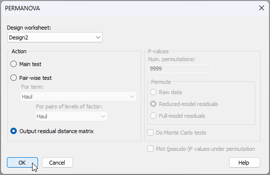
Notice here, in passing, that the right-hand side of the dialog is 'greyed out' when we choose the option to output a residual distance matrix, as no permutations or tests need to be done in that case. Click 'OK'.

The residual distance matrix is output as 'Resem2' in the Explorer tree, as shown below:

Finally, we are ready to take a look at our multivariate residuals in an ordination diagram. From 'Resem2', click Analyse > MDS > Nonmetric MDS (nMDS).... Accept all of the defaults in the 'Non Metric MDS' dialog and just click 'OK'. Once the default plot has been produced, click Graph > Sample Labels & Symbols... and choose the Labels to be plotted according to the factor of 'Haul', and the Symbols to be plotted according to the factor of 'Position', just as we had done before.

The resulting lowest-stress 2D nMDS solution for our residual ordination plot (having removed effects due to 'Haul') looks like this:

This is very different from the plot we saw before! Now the effects due to the 'Position' are abundantly clear! This might seem like a spot of magic, but if you sneak a peek back at the original nMDS plot (above), you might notice that, for most of the pairs of observations within a given haul, the 'U' (blue) symbol occurs to the left of the 'L' (amber) symbol. Thus, when we center all of the haul pairs (1 through 10) onto a common centroid, the blue symbols appear to the left and the amber symbols appear to the right. Of course, don't forget that the centering (i.e., the calculation of residual distances) is done in the full-dimensional space, and not in the 2d nMDS space. Being able to carefully work out the patterns we see in a residual plot for a given factor by reference to the original plot in this way is not always possible, however. In fact, it will rarely be the case, as typically the effects of factors are happening across a lot more than 2 dimensions. Nevertheless, this example definitely shows us this fantastic tool for visualising minor effects after removing the effects of some other factor(s) or nuisance variable(s).

^‡In this particular example, however, ANOSIM cannot be used for the test of Position for the two-way crossed design, because there is no replication within the cells of the design (i.e., within the Position-by-Haul combinations) and the Position factor has fewer than 3 groups.

^¶This is a case of a two-way unreplicated ANOVA design. The lack of replicate nets at the same depth for each haul means that we will be unable to partition out and estimate any potential Position$\times$Haul interactive effects from the estimated Residual variation, with which it is confounded. Despite this inability to separately test for an interaction, it is still important, nevertheless, to fit a two-way design here that includes the 'Haul' factor, and not to fit a one-way model with only the 'Position' factor alone. Specifically, if we ignore the paired nature of the nets in the sampling protocol, we risk being unable to detect 'Position' effects at all. See the section on unreplicated designs in the original PERMANOVA+ manual for details.

^†In this particular case (i.e., a one-way PERMANOVA), it does not matter whether we specify 'Haul' as being fixed or random; the residuals will be the same either way. We specify it as random here for clarity and consistency in the specification of our reduced (one-factor) model.