6. Allow heterogeneous dispersions in PERMANOVA
- 6.1 Overview - Allow heterogeneity
- 6.2 ANOVA in a nutshell
- 6.3 The Behrens-Fisher problem (BFP)
- 6.4 Multivariate Behrens-Fisher problem
- 6.5 Solution to the multivariate BFP
- 6.6 Example: one-way PERMANOVA allowing heterogeneity
- 6.7 Heterogeneity in more complex designs
- 6.8 Example: two-way crossed PERMANOVA allowing heterogeneity
6.1 Overview - Allow heterogeneity
An important assumption of classical analysis of variance (ANOVA) is that the errors come from a distribution with a common variance. By this we assume, in essence, that the variability of the sampling units within each group is constant and equivalent across all of the groups. Similarly, for mulivariate dissimilarity-based tests, such as PERMANOVA ( Anderson (2001) ), we generally wish to assume that the dispersion (spread) of the sampling units in the space of the chosen resemblance measure is consistent across the groups. A PERMDISP test may be used to ascertain homogeneity of multivariate dispersions formally ( Anderson (2006) ). In the absence of heterogeneous dispersions, any significant result that may arise from our PERMANOVA test can be attributed to a shift in centroid. The effects of heterogeneity of multivariate dispersions on inferences in PERMANOVA tests were found only to be of some consequence in the case of unbalanced designs, and these effects were nowhere near as dramatic for PERMANOVA as they were for ANOSIM or Mantel tests ( Anderson & Walsh (2013) ).
Anderson et al. (2017) have provided a modification to the original PERMANOVA pseudo $F$ test statistic that allows heterogeneity of dispersions. The new PERMANOVA routine in PRIMER 8 can be used to implement this technique, permitting the end-user to make direct inferences regarding differences in centroids, while taking into account known heterogeneity in dispersions, where present.
This chapter begins with a short description of ANOVA and the Behrens-Fisher problem (BFP) for univariate cases, then describes the BFP for multivariate situations. The solution to the multivariate BFP provided by Anderson et al. (2017) is then given, and we step through a one-way example. Complications that arise when we move to consider more than one factor in multi-way ANOVA designs are then discussed. We then step logically through a two-way example to clarify these ideas, outlining appropriate tests and associated graphics in a case study.
6.2 ANOVA in a nutshell
The one-way ANOVA model
In one-way univariate analysis of variance (ANOVA), interest lies in comparing the means among several groups. More formally, ANOVA tests the null hypothesis of no differences in the population means among groups.
Let $y_{ij}$ be the $j$th observation for variable $Y$ in the $i$th group, with $i = 1, \ldots, a$ groups and $j = 1, \ldots n_i$ observations per group. The ANOVA linear model is: $$ y_{ij} = \mu + \alpha_i + \varepsilon_{ij} $$ where $\mu$ is the overall population mean parameter, $\alpha_i$ is the population group effect parameter for a particular group $i$ and $\varepsilon_{ij}$ is the error parameter associated with $y_{ij}$, the $j$th observation in group $i$. The population means for each group $i$ can be defined as: $$ \mu_i = \mu + \alpha_i $$
and our null hypothesis in ANOVA is that all of the population group means are equal to one another, written formally as: $$ \text{H}_ 0 : \mu_1 = \mu_2 = \ldots = \mu_a $$ or, equivalently, that all of the population group effect parameters are equal to zero: $$ \text{H}_ 0: \alpha_1 = \alpha_2 = \ldots = \alpha_a = 0. $$
Although interest lies in the comparison of means, it is possible that the groups differ from one another in other ways as well. For example, the groups may have different variances; that is, the spread or dispersion of the observations occurring within each group may differ from one another, with some groups being more spread out/dispersed than others. We may denote the population variances associated with the errors belonging to any particular group $i$ as $\sigma^2_i$.
The F ratio
The test statistic used in ANOVA is a ratio of two mean squares. Specifically the classical univariate $F$ ratio for the one-way ANOVA case may be defined as:
$$
F = \frac{ \sum_{i=1}^a n_i(\bar{y}_ {i\cdot} - \bar{y}_ {\cdot\cdot})^2 / (a - 1) }
{ \sum_{i=1}^a (n_i - 1) s_i^2 / (N - a) }
$$
where
$ \hspace{1cm} N = \sum_{i=1}^a n_i \hspace{0.05 cm}$, the sum of all observations;
$ \hspace{1cm} \bar{y}_ {i\cdot} = \sum_{j=1}^{n_i} y_{ij}/n_i \hspace{0.05 cm}$, the sample mean of group $i$;
$ \hspace{1cm} \bar{y}_ {i\cdot\cdot} = \sum_{i=1}^a \sum_{j=1}^{n_i} y_{ij} / N \hspace{0.05 cm}$, the sample mean of all observations; and
$ \hspace{1cm} s_i^2 = \sum_{j=1}^{n_i} (\bar{y}_ {ij} - \bar{y}_ {i\cdot})^2 / (n_i - 1) \hspace{0.05 cm}$, the sample standard deviation of group $i$.
For the one-way case, we can think of $F$ as a ratio of two measures of variation: the among-group mean square in the numerator measures the variation among the groups; the within-group mean square in the denominator measures the variation within the groups.
Assumptions of classical ANOVA
In addition to the linear model itself (articulated above), classical ANOVA asserts the following (three-part) assumption to maintain the validity of the $F$ test:
- The errors, $\varepsilon_{ij}$, are independent and identically distributed random variables, drawn from a normal distribution with a mean of $0$ and a common variance of $\sigma^2_\varepsilon$.
We may write the 'common variance' (or 'homogeneity of variances') aspect of this assumption as a statement that all of the within-group variances are equal to one another: $$ \sigma^2_1 = \sigma^2_2 = \ldots = \sigma^2_a $$
Calculating a p-value
If the null hypothesis is true, and all of the assumptions above are fulfilled, then $F$ is a random variable distributed as $F_0$, a ratio of two chi-square random variables, having degrees of freedom $(a - 1)$ and $(N - a)$ in the numerator and denominator, respectively; i.e., $$ F \sim F_0 = \frac{X_\text{num}}{X_\text{denom}} $$ where $$ X_\text{num} \sim \chi^2_{(a-1)} \hspace{1cm} \text{and} \hspace{1cm} X_\text{denom} \sim \chi^2_{(N - a)} $$
By knowing this distribution, the p-value for the test can then be calculated directly for any observed value $F_{\text{obs}}$ calculated from data, as follows: $$ P = \text{Pr}(F_0 \ge F_{\text{obs}}) $$
Test by permutation
We can rather easily dispense with the assumption of normality altogether, however, by using a permutation test. For example, if we ran a PERMANOVA on univariate data (based on Euclidean distances), then we would obtain a classical ANOVA partitioning and associated $F$-ratio test-statistic, but with the p-value calculated empirically using permutations. In that case, we do not assume normality (or any other distribution), but only exchangeability of the observations among the groups under a true null hypothesis.
Specifically, we calculate the observed value of $F$ for the original data, $F_\text{obs}$, then we randomly shuffle (permute) and re-allocate all of the $N$ observations across all of the groups, maintaining the original sample size $n_i$ for every group $i$. After the re-allocation, we get a value of $F$ under permutation, $F^{\pi}$. We repeat this random re-allocation and re-calculation of $F$ under permutation many times to get an entire permutation distribution of values of $F^{\pi}$ under the null hypothesis of no differences among the groups, i.e., all observations $y_{ij}$ are exchangeable. The p-value under permutation is then calculated empirically by tallying the number of $F^{\pi} \ge F_{\text{obs}}$ and looking at this as a proportion of the total number of permutations done, $n_\text{perm}$: $$ P = \frac{( \text{no. of } F^{\pi} \ge F_{\text{obs}} ) + 1}{ (n_\text{perm} + 1) } $$
Note that '$+1$' in the numerator and denominator acknowledge the observed value $F_{\text{obs}}$ as a member of this distribution (being one possible realised allocation). If we systematically do all possible re-allocations (in which case the '$+1$' in the numerator and denominator of the above equation would not be needed), then the resulting empirical permutation p-value is exact.† If we do a random sub-set of all possible permutations, then we get an estimate of the p-value that is nevertheless accurate (unbiased), and it gets more and more precise, the larger the value of $n_\text{perm}$ we are able to achieve.
Violations of assumptions
Independence of the errors is typically not difficult to achieve in practice, simply by taking care with the study design itself and the way observations are sampled (e.g., using random representative sampling). A thoughtful discussion of the consequences of non-independence (positively or negatively, either within or among groups) is provided by Underwood (1997) .
Normality of the errors is typically much more difficult to fulfill; however violation of this assumption does not typically have a strong impact on the validity of the test. Even if errors are not normally distributed, the central limit theorem ensures that the distribution of means will be approximately normal, and the ANOVA $F$ test remains quite robust. Also, the use of a permutation test to calculate the p-value avoids having to make this particular assumption.
The assumption of homogeneity of variances across all groups is also rather easy to violate in practice. For example, count data (such as the abundances of a species) typically show intrinsic mean-variance relationships, so any differences in means among groups will almost surely be accompanied by differences in variances as well ( McArdle & Anderson (2004) ). The assumption of homogeneity of variances across all groups, if violated, will not affect the validity of the test appreciably provided the design is balanced; i.e., if there are equal sample sizes across the groups. However, if the design is unbalanced, then heterogeneity of variances will potentially affect either the Type I error rate or the Type II error rate of the test, depending on the nature of the heterogeneity.¶
Effects of heterogeneity (univariate)
In classical univariate ANOVA, in cases where there is heterogeneity of variances and the design is unbalanced, then:
- if there is greater dispersion in one or more groups that have a small sample size, then the tendency will be to inflate the Type I error of the ANOVA test;
- if there is greater dispersion in one or more groups that have a large sample size, then the tendency will be to inflate the Type II error of the ANOVA test.
For more details of these effects, see Welch (1938) , Horsnell (1953) , Box (1954) and Glass et al. (1972) .
Permutation tests do not provide a solution to this issue. They, too, are sensitive to differences in dispersion; groups with different dispersions cannot strictly be considered to be 'exchangeable' under a true null hypothesis of no differences in means (e.g., see Boik (1987) and Hayes (1996) ).
What is needed is a method for testing differences in means when variances differ.
¶Recall that:
- the probability of a Type I error is the probability of rejecting H0 when it is true; and
- the probability of a Type II error is the probability of failing to reject H0 when it is false.
† By an exact test, we mean that the Type I error of the test is exactly equal to the a priori chosen significance level of the test. For an exact test, if you choose a significance level of (say) 0.05, and you reject the null hypothesis any time you get a p-value less than or equal to 0.05, then the probability that you will reject a true null hypothesis is indeed precisely 0.05; that is, you will be wrong 5% of the time.
6.3 The Behrens-Fisher problem (BFP)
Overview
The Behrens-Fisher problem (BFP) is one of the oldest puzzles in statistics ( Behrens (1929) ; Fisher (1935) ; Welch (1938) ). The essence of this problem is how validly to compare the means of two or more populations (groups) when their variances differ. It is clear how the assumption of common variance is built right in to the ANOVA $F$ statistic itself. For example, consider the one-way case, where the $F$ ratio is built using a single common estimate of the error variance (i.e., the residual mean square) as its denominator.
There are quite a few solutions to the Behrens-Fisher problem for univariate data (e.g., see Wang (1971) , Brown & Forsythe (1974) , Clinch & Keselman (1982) , Weerhandi (1993) and Ghosh & Kim (2001) ), yet all generally assume normality of errors.
Below we shall outline a solution to the univariate BFP proposed by Brown & Forsythe (1974) , as it points the way towards a more generalised solution to the BFP for multivariate data in dissimilarity-based analyses, using PERMANOVA.
The Brown & Forsythe (1974) solution to the BFP
Brown & Forsythe (1974) proposed a modification of the classical univariate $F$ ratio such that the means are weighted by $n_i / s_i^2$ (rather than being weighted only by $n_i$) and the denominator is chosen in order to ensure that numerator and denominator have the same expectation under a true null hypothesis, after this adjustment in the weights.
The resulting modified test-statistic is given by them as: $$ F_{\tiny{BF}} = \frac{ \sum_{i=1}^a n_i (\bar{y}_ {i \cdot} - \bar{y}_ {\cdot\cdot})^2 } { \sum_{i=1}^a (1 - n_i / N) s_i^2 } $$ Under the usual classical ANOVA assumptions, a p value can be obtained by comparing this modified test-statistic to an $F_0$ distribution having $(a-1)$ and $f$ degrees of freedom (defined implicitly by the Satterthwaite (1941) approximation), where: $$ f = \frac{1} { \sum_{i=1}^a c_i^2 / (n_i - 1)} $$ and $$ c_i = \frac { (1-n_i/N)s_i^2 } { \sum_{i = 1}^a (1 - n_i/N)s_i^2 } $$
Next, we shall see how a similar modification to the PERMANOVA pseudo F statistic can be constructed to allow heterogeneous dispersions in dissimilarity-based settings as well.
6.4 Multivariate Behrens-Fisher problem
Overview
In a multivariate context, there are many ways that groups of sampling units can differ from one another. For example, let's consider conceptually just three important ways that groups (i.e., sets of sampling units in a multivariate space) can differ from one another (see Fig. 6.1). (There are more ways, of course)! They can differ in the position of their central location (centroids), in the overall variability of their sampling units (dispersion or spread), and/or in their degree of correlation among pairs of variables (shape).
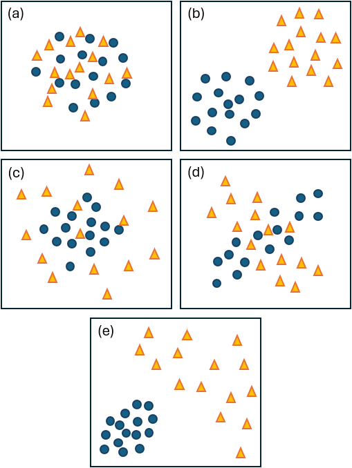
Fig. 6.1. Schematic diagram of bivariate data in each of two groups (triangles vs circles) where the groups have: (a) similar centroids, spread and shape; (b) different centroids (a shift in the central location of the points); (c) different spread (triangles are more dispersed); (d) different shapes (triangles show a pattern of negative correlation, while circles show a pattern of positive correlation); and (e) different centroids, different overall spread and different shapes.
The multivariate Behrens-Fisher problem in classical statistics is typically stated as the problem of testing for the equality of mean vectors (centroids) from two or more multivariate normal distributions (groups or populations), when their covariance matrices (describing the shape and dispersion of the samples within each group) are possibly not equal.
The majority of solutions to the multivariate BFP (e.g., see Johnson & Weerhandi (1988) , Coombs & Algina (1996) , Christensen & Rencher (1997) , Gamage et al. (2004) , Belloni & Didier (2008) , Krishnamoorthy & Lu (2010) ) assume variables are multivariate normal and also do not handle high-dimensional data, where the number of variables can exceed the sample sizes (but see Ahmad et al. (2012) and Ahmad (2014) for some proposed non-parametric solutions to the multivariate BFP based on U statistics).
However, we would really like a solution to the multivariate BFP for dissimilarity-based approaches (such as ANOSIM or PERMANOVA). In this context, the somewhat more general multivariate BFP would be stated as:
- How can we test for differences in central location (in the multivariate space defined by a given resemblance measure) when there are differences in dispersion (spread) among the groups?
We may begin by doing a test for homogeneity of multivariate dispersions using the PERMDISP routine in PRIMER (see Anderson (2006) and Anderson et al. (2006) ). If we find significant differences in spread among the groups, then we may consider how this might affect any test we may wish to perform using either ANOSIM or PERMANOVA.
Effects of heterogeneous dispersions on dissimilarity-based tests
ANOSIM
Anderson & Walsh (2013) did a simulation study to investigate how ANOSIM and PERMANOVA would be affected by variation in multivariate dispersions. They found that ANOSIM was very strongly affected by heterogeneity. Specifically, the ANOSIM test is sensitive to:
- differences in location (centroids);
- differences in dispersion; and/or
- differences in shape.
ANOSIM's null hypothesis may be put simply as 'there are no differences among the groups', so any of these types of differences (individually or collectively), might trigger a significant result in an ANOSIM test. Although ANOSIM is more likely to reject the null hypothesis for changes in location (centroid), it does not set out to be a test for differences in location only - it is a test of any differences between groups that might render them 'distinctive'. Indeed, the R statistic in ANOSIM might best be regarded as a measure of the distinctiveness of the groups (see Clarke (1993) and Warwick & Clarke (1993) ).
PERMANOVA
In contrast, PERMANOVA is much more akin to classical ANOVA. It performs a partitioning of the variability in the space of the resemblance measure, and therefore is focused much more strongly on detecting shifts in location. PERMANOVA tests the more specific null hypothesis: 'there are no differences among the group centroids' in that space. The behaviour of PERMANOVA in the face of heterogeneous dispersions also mirrors what has been found for the classical univariate $F$ test. Specifically, Anderson & Walsh (2013) found that PERMANOVA was not affected by heterogeneous dispersions if the design was balanced (equal sample sizes per group). However, if the design was unbalanced (unequal sample sizes per group), then, precisely as in a univariate $F$ test, PERMANOVA was:
- conservative (yielding an inflated Type II error rate) if a group (or groups) with a large sample size also had large variation relative to other groups; and
- liberal (yielding an inflated Type I error rate) if a group (or groups) with a small sample size also had large variation relative to other groups.
In other words, if a group with a large sample size is greatly dispersed, then it wil be very difficult to detect a true shift in the centroids; the large within-group dispersion of that group will dominate the analysis (Fig. 6.2a). On the other hand, if a small sample-sized group has large dispersion, then even small differences in the sample centroids entirely due to random sampling might look relatively large (and be detected as significant) relative to the small within-group dispersion seen in other groups (Fig. 6.2b).
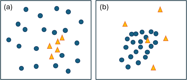
Fig. 6.2. Schematic diagram showing how imbalance can affect tests for differences in centroid in PERMANOVA: (a) large dispersion in a group with a large sample size will increase Type II error, hence decrease the power of the test; (b) large dispersion in a group with a small sample size will increase Type I error.
6.5 Solution to the multivariate BFP
Overview
Anderson et al. (2017) described a general dissimilarity-based solution to the multivariate Behrens-Fisher problem. Their solution uses a statistic (called '$F_2$' therein) that is a modification of the original PERMANOVA pseudo F statistic (called '$F_1$' therein). This modification is a direct dissimilarity-based multivariate analogue to a solution to the univariate BFP proposed by Brown & Forsythe (1974) . The PERMANOVA routine in PRIMER is the only known software implementation of this method that correctly accounts for heterogeneity in multivariate dispersions not only in the construction of the test-statistic itself, but also in the algorithm used for permutations to estimate the p-value.
What is described below are the details of the one-way case, but for more complex ANOVA designs with multiple factors, the end-user must specify wherein the heterogeneity lies that needs to be accounted for, and the construction of the correct $F$ statistic and associated permutation algorithm required to achieve rigorous inference in the context of the full study design is not trivial. We re-iterate: the PERMANOVA routine in PRIMER is the only software we know of that will do all of this correctly.
PERMANOVA in a nutshell
For a description of PERMANOVA, please see the original articles ( Anderson (2001) , McArdle & Anderson (2001) ) and also the rather more recent and more thorough encyclopedia entry provided by Anderson (2017) . We shall describe the original PERMANOVA test-statistic here, in brief, following Anderson et al. (2017) , with notation that facilitates the description of the modified test.
Suppose $\bf Y$ is an $N \times p$ matrix of multivariate row vectors ${\bf y}_ {ij}$ corresponding to sampling units, each of length $p$ and each belonging to one of $i = 1, \ldots, a$ groups, with $j = 1, \ldots, n_{i}$ sampling units (rows) in the $i$th group and $N = \sum_{i=1}^a n_i$. Let $\bf D$ be an $N \times N$ symmetric matrix of dissimilarities $\lbrace d_{ij,i'j'} \rbrace$ calculated between every pair of sampling units.
Next, as in Gower (1966) , let matrix $\bf A$ be comprised of elements $\lbrace a_{ij,i'j'}\rbrace$ = $\lbrace -0.5 \times d_{ij,i'j'}^2 \rbrace$, then define matrix $\bf G$ (a centred version of matrix $\bf A$) as: $$ {\bf G} = ( {\bf I} - (1/N) {\bf J}_ {\scriptscriptstyle N} ) {\bf A} ( {\bf I} - (1/N) {\bf J}_ {\scriptscriptstyle N} ) $$ where ${\bf J}_ {\scriptscriptstyle N}$ denotes an $N \times N$ matrix of $1$s and $\bf I$ denotes an $N \times N$ identity matrix.
For the one-way case, let $\bf X$ be a $N \times r$ matrix of full rank $r = (a-1)$ containing orthogonal contrasts among the groups. We can construct a linear projection matrix for the design as: $$ {\bf H} = {\bf X} [ {\bf X}'{\bf X} ]^{-1} {\bf X}' $$ Then, the PERMANOVA pseudo $F$ statistic for comparing the centroids among the $a$ groups is: $$ F_1 = \frac { \text{tr} ({\bf HG})/(a-1) } { \text{tr} [ {\bf (I-H) G} ] /(N-a) } $$
where '$ \text{tr}(\cdot)$' denotes the trace (sum of diagonal elements) of a matrix. Note that if $p = 1$ and $\bf D$ is calculated using Euclidean distances, then $F_1 = F_0$, the classical univariate $F$ ratio.
Test by permutation
We may calculate a p-value to test the null hypothesis of equality of centroids in the space of the chosen dissimilarity measure under the sole assumption that the sampling units (rows) are exchangeable among the $a$ groups. First, we calculate an observed value of the test statistic, $F_1$, with the rows of the data (sampling units) in their original order. Then, we randomly permute (re-order) the $1,\ldots,N$ rows of matix $\bf Y$ to obtain a matrix of permuted data ${\bf Y}^\pi$, yet leaving the grouping structure fixed (i.e., the original ordering is retained in matrix $\bf X$ and hence also in the projection matrix $\bf H$). In other words, under a true null hypothesis, any ordering of the sampling units across the groups is equally likely via exchangeability. Indeed, exchangeability is the only assumption of the PERMANOVA test, which is distribution-free.
Re-calculation of $F_1$ replacing $\bf Y$ with ${\bf Y}^\pi$ yields $F_1^\pi$, a value of the test-statistic under permutation. Repeating this random permutation and re-calculation a large number of times (say, $n_\text{perm} = 9999$), yields a distribution of values of $F_1^\pi$ from which we can empirically calculate a p-value as $P = \text{Pr}(F_1^\pi \ge F_1)$. Specifically, the p-value is calculated directly as:
$$ P = \frac{( \text{no. of } F_1^{\pi} \ge F_1 ) + 1}{ (n_\text{perm} + 1) } $$
This mirrors what we saw for the test by permutation for univariate ANOVA (and so many other permutation tests offered in PRIMER); namely, that the $+1$ in each of the numerator and denominator are there simply to acknowledge the inclusion of the original (genuine) ordering of the data as one of the possible 'random' outcomes we could have obtained - they would not be needed in the equation if all possible orderings were to be done systematically and exhaustively.
Modified PERMANOVA to account for heterogeneity
Anderson et al. (2017) suggested a modification to the PERMANOVA pseudo $F$ statistic to account for heterogeneity, following directly from the univariate solution to the BFP proposed by Brown & Forsythe (1974) . Specifically, instead of $F_1$, we can use:
$$ F_2 = \frac { \text{tr} ({\bf HG}) } { \sum_{i=1}^a (1-n_i/N) \cdot V_i } $$
where $V_i$ is the within-group dispersion for group $i$, defined as:
$$ V_i = \sum_{j=1}^{(n-1)} \sum_{j'=(j+1)}^n d_{ij,i'j'}^2 / [ n_i(n_i-1) ] $$
Some important things to note about this modified test-statistic are:
- The null hypothesis for $F_2$ is equality of centroids in the space of the chosen dissimilarity measure given potential differences in dispersions among the groups.
- The potential for heterogeneity is explicitly acknowledged in the modified test-statistic, $F_2$ by the calculation of separate individual dispersions ($V_i$) for each group.
- $F_2$ is equivalent to $F_1$ if sample sizes are equal across all groups. This is sensible, as PERMANOVA (like ANOVA) is very robust to heterogeneity of dispersions when the design is balanced.
- $F_2$, like $F_1$, is carefully constructed so that the numerator and denominator have the same expectation when the null hypothesis is true.
- If we are dealing with univariate data, so $p = 1$ response variable, and the entries in ${\bf D}$ are Euclidean distances, then $V_i$ is the usual classical univariate unbiased measure of the sample variance ($s^2$) for group $i$.
- If PERMANOVA is run using $F_2$, then the degrees of freedom are also modified to reflect the Satterthwaite approximation given by Brown & Forsythe (1974) . This is to ensure compatibility between the PERMANOVA implementation and the solution provided by Brown & Forsythe (1974) for univariate cases, but in practice the p-value itself is always calculated in PERMANOVA using permutation algorithms (see below), so there is no direct consequence of this change in the degrees of freedom (which will remain constant under permutation) for the level of significance in the outcome.
Obtaining a p-value for the modified test
On the face of it, we would not expect to be able to do a permutation test for $F_2$, because how can we view the sampling units as exchangeable among the groups if we know already that the groups have different dispersions? Some alternative method, such as a separate-sample bootstrap, either with or without some kind of bias-adjustment (e.g., Efron & Tibshirani (1993) , Manly (2006) ), would seem to be more appropriate to use here, at least conceptually. Simulation work by Anderson et al. (2017) demonstrated, however, that the modified test based on $F_2$ had better statistical behaviour when permutations were done to obtain the p-value, rather than bootstraps. To be specific, the Type I error was closer to the nominated significance level and the distribution of p-values under a true null hypothesis was more uniform (as is desirable) when tests were done using permutations. In contrast, the results obtained using bootstrapping methods were always much more conservative, and the degree of conservatism increased with increasing dimensionality, increasing degree of heterogeneity and increasing differences in sample sizes among groups. In addition, under all simulation scenarios, tests by permutation using $F_2$ had the greatest power, matching or exceeding that of $F_1$, compared to bootstrap alternatives.
Thus, PERMANOVA in PRIMER that is done using $F_2$ to account for heterogeneity calculates p-values using permutation algorithms rather than using bootstrapping methods.
6.6 Example: one-way PERMANOVA allowing heterogeneity
Let's look now at an example where there is a single factor in the study design, the number of replicates per group is unequal and there is clear heterogeneity in multivariate dispersions among the groups. Ellingsen & Gray (2002) studied the biodiversity of soft-sediment macrobenthic organisms and its relationship with environmental variation over large spatial scales in the North Sea. Samples of soft-sediment macrobenthic organisms were obtained from $N$ = 101 sites occurring in five large delineated areas along a transect spanning 15 degrees of latitude (Fig. 6.4). The sample sizes in the five areas were: $n_1$ = 16, $n_2$ = 21, $n_3$ = 25, $n_4$ = 19 and $n_5$ = 20. A total of $p$ = 809 taxa were recorded overall, and samples consisted of abundances pooled across five benthic grabs obtained at each site.
Interest lies in comparing the multivariate assemblages of organisms occurring in these five areas. More specifically, we wish to use PERMANOVA to test the null hypothesis:
- H0: there are no differences in the centroids of these 5 areas in the space of the Jaccard resemblance measure, allowing for any potential heterogeneity in the within-group dispersions among these areas.
In ecology, the Jaccard measure is directly interpretable as the percentage of shared species between every pair of sampling units. When expressed as a dissimilarity, it is often used as a pure measure of turnover in studies of beta diversity ( Anderson et al. (2006) ).
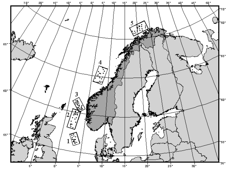
Fig. 6.4. Map showing locations of sites in each of 5 areas in the North Sea from which macrobenthic fauna were sampled (after Ellingsen & Gray (2002) ).
Open the data in PRIMER and examine patterns
- Start running PRIMER 8, then click File > Open... to open the data file named 'Norway_macrofauna.pri' (found inside the 'Examples_P8 > Norway_macrofauna' folder).
![05.Norway_data_in_PRIMER[i].png](https://learninghub.primer-e.com/uploads/images/gallery/2025-12/05-norway-data-in-primer-i.png)
- Get the resemblance matrix among the sampling units based on the Jaccard measure. Click Analyse > Resemblance... > (Measure > $\bullet$ Other) and from the drop-down list choose 'S7 Jaccard'.
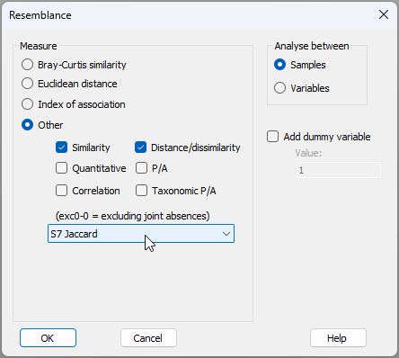
The resulting resemblance matrix will be called 'Resem1'.
- To visualise the inter-sample relationships based on the identities of the fauna they contain, obtain a non-metric multi-dimensional scaling (nMDS) ordination plot based on the Jaccard resemblances. From the 'Resem1' similarity matrix, click Analyse > MDS > Non-metric MDS (nMDS)..., take the default options and click 'OK'. This will generate the following 2D ordination plot (called 'Graph1'), or a highly similar solution¶:
![06.nMDS_normac_E&G[i].png](https://learninghub.primer-e.com/uploads/images/gallery/2025-12/06-nmds-normac-eg-i.png)
Perhaps the most striking pattern here is the tight clustering of samples from Area 1 (low dispersion) and the very large spread of the samples from Area 3 (high dispersion), compared to Areas 2, 4 and 5.
Test for homogeneity of multivariate dispersions
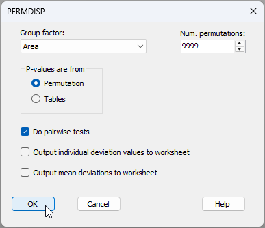
- Although it is fairly obvious from the graphic, let's test the null hypothesis of no differences in the within-group dispersions among the five areas using PERMDISP. From the 'Resem1' similarity matrix, click PERMANOVA+ > PERMDISP... > Group factor: Area (leaving the rest as their defaults) and click 'OK', as shown below:
The results are given in the file 'PERMDISP1' of the Explorer tree (see below).
![08.PERMDISP_results_normac[i].png](https://learninghub.primer-e.com/uploads/images/gallery/2025-12/08-permdisp-results-normac-i.png)
There are clearly highly significant differences in the dispersions among the groups ($F$ = 49.778, $P$ = 0.0001 with 9999 permutations). The pairwise tests, furthermore, reveal how Area 1 and Area 3 differ significantly from one another and from the other three groups (2, 4 and 5) with respect to their dispersions, reflecting rather directly the patterns of differences in spread we observed in the nMDS plot.
Test for differences in centroids, allowing for heterogeneity
Having observed these dispersion differences among the areas - quite interesting differences in themselves - we now aim to test for diferences in centroids, allowing for that heterogeneity. Running a PERMANOVA requries two steps: (i) setting up a design file; and (ii) running the PERMANOVA analysis on a given data set in response to a specified design.
- From the 'Resem1' similarity matrix, create the design file by clicking PERMANOVA+ > Create PERMANOVA Design.... You will see a new item named 'Design1' (symbolised by
![09.Design_file_icon[i].png](data:image/png;base64,iVBORw0KGgoAAAANSUhEUgAAABEAAAAQCAIAAAB/UwMIAAAAAXNSR0IArs4c6QAAAARnQU1BAACxjwv8YQUAAAAJcEhZcwAADsMAAA7DAcdvqGQAAAASdEVYdFNvZnR3YXJlAEdyZWVuc2hvdF5VCAUAAAGJSURBVDhPnZLBSwJBFMb9f/ag0K3w7q17l47R3UPQRaiT5JpiJGUWhqMxstoWHkowiDLDk+tqelEW9iKiyLqrs+OMESO7bQhRH+/w3sz3m/cdxrX4u1w/ZkJIv9//aLc7nc54PP5xy2QzlNJK9W0zG+FE3qoDcDEajRyExRBCYjD93W2VNx9VVXUFU3oqW6YtEA1kEj5oL/TBiGEYDgZj7IUhTuS3MzFVVQkh0+mUEPL8+uIWggwDYt7BKIrCibxbCA6HQ7nZZBv8ID6ZTErl5X4PDJumaTPNVosT+QBIIoQ8MGxFOgRJjPF6fhlSURSb6fV6nMiHbq50XedEfu3+WCjeMR9CaB+cs77ZatnMbDZzC0EvDBmG0ZDlhixrmsZ8pmn6QZz13W7XZhaLRaqQ40R+B5zWJUmW5d3rk6+0mQTG2Eqr67qDQQhZ77HagEeDwaBSrbLRD+LM6fgH8/n8vVaLwXQwe1l8fNA0jVK6B84YU5ekFcxKYYzTt0KqkKOUWoe/MCv1H+YThTyXobX3/k4AAAAASUVORK5CYII=) )
in the Explorer tree.
You will need to do the following:
)
in the Explorer tree.
You will need to do the following:
![09.Design_file_icon[i].png](https://learninghub.primer-e.com/uploads/images/gallery/2025-12/09-design-file-icon-i.png)
- Click the white cell in the first column under the word 'Factor' and choose: 'Area' as the sole factor of interest for this design. (Note in passing that the default is to treat this factor as 'Fixed', as shown under the word 'Type' in the third column of the design file, which is fine here).
- Under 'Dispersions', tick the box $\checkmark$ 'Allow for heterogeneity', then click the
 button.
 - In the resulting dialog box entitled 'Select the term identifying groups with different dispersions' choose 'Area'.

![09c.Groups_dialog_normac[ii].png](https://learninghub.primer-e.com/uploads/images/gallery/2025-12/09c-groups-dialog-normac-ii.png)
Your resulting design file should look like this:
![10.Design_file_for_normac[ii].png](https://learninghub.primer-e.com/uploads/images/gallery/2025-12/10-design-file-for-normac-ii.png)
Note that by ticking the box $\checkmark$ 'Allow for heterogeneity', we ensure that the PERMANOVA tests will be done using $F_2$ rather than $F_1$ for all tests of relevant terms affected by the heterogeneity we have identified using the 'Groups' button.
- Now that you have created the design file, you are ready to run the analysis itself. We're going to test the null hypothesis of no differences in the centroids among the five areas using PERMANOVA and allowing for heterogeneity in dispersions. Go back to the 'Resem1' similarity matrix and, from there, click PERMANOVA+ > PERMANOVA.... In the PERMANOVA dialog window:
- Under the words 'Design worksheet:' make sure you choose the name of the correct design file, i.e. 'Design1'.
- Under the word 'Action', choose $\bullet$ Main test.
- Under the word 'Permute' choose $\bullet$ Raw data (because there is only one factor here).
- Optionally, you can choose to tick the box to $\checkmark$ 'Plot (pseudo-)F values under permutation'. The rest of the items in the dialog can remain as the defaults (see below), then click 'OK'.
![11.PERMANOVA_dialog_normac[i].png](https://learninghub.primer-e.com/uploads/images/gallery/2025-12/11-permanova-dialog-normac-i.png)
The resulting PERMANOVA output file ('PERMANOVA1', shown below) indicates strong evidence against the null hypothesis of no differences in the centroids among these five areas ($F_2$ = 13.51, $P$ = 0.0001 with 9999 permutations). So, not only are there differences in the variability of the assemblages (evidenced by the PERMDISP analysis), there are also clear shifts in centroid evidencing overall turnover in the identities of species across these five areas (also apparent in the nMDS plot above).
![12.PERMANOVA_Main_output[i].png](https://learninghub.primer-e.com/uploads/images/gallery/2025-12/12-permanova-main-output-i.png)
It is worth noticing a couple of things about the PERMANOVA output file that makes it different from what would be obtained if we did not allow for heterogeneity. Specifically:
- The expectation of the mean square for 'Area' includes linear combinations involving separate individual measures of residual variation for each of the five areas. In other words, we do not have a single pooled estimate of error variance at work here, but an explicit recognition of the different within-group dispersions.
- The denominator degrees of freedom for the test of 'Area', therefore, is not a whole number, but instead this value is drawn directly from the theory for this arising from the univariate solution to the Behrens-Fisher problem described by Brown & Forsythe (1974) . As previously discussed, this has no direct consequence on the test by permutation using $F_2$ for the multivariate setting, but it does point to the fact that the power of the test using $F_2$ may well differ from that using $F_1$ (which perfectly stands to reason, as they are actually testing different hypotheses).
- Having found a significant result for the main test in PERMANOVA, it is now desirable to run pair-wise comparisons that also will account for heterogeneity. We simply re-run the PERMANOVA routine from the same resemblance matrix, pointing to the same design file ('Design1'), but this time, under the word 'Action', we choose $\bullet$ Pair-wise test > For term: 'Area' > For pairs of levels of factor: 'Area', like this:
![11.PERMANOVA_dialog_normac_pairwise[i].png](https://learninghub.primer-e.com/uploads/images/gallery/2025-12/11-permanova-dialog-normac-pairwise-i.png)
Our results file for the pair-wise tests ('PERMANOVA2') will then appear as follows:
![13.PERMANOVA_Pairwise_output_normac[i].png](https://learninghub.primer-e.com/uploads/images/gallery/2025-12/13-permanova-pairwise-output-normac-i.png)
In passing, we can see how using $F_2$ on the pairwise tests creates differences from what we would see for a PERMANOVA using $F_1$ on these data. These differences essentially mirror what we saw for the main test; namely, there are separate individual measures of residual variation for each area, and there are also non-integer denominator degrees of freedom for each test.
Overall, from this study, we can conclude that there are highly significant differences in the identities of species obtained from each of these five different areas - they clearly contain different sorts of soft-sediment benthic assemblages. This is so despite the very large variation in the assemblages inhabiting different sites sampled from Area 3. Our tests accounted for that.
It is obviously very satisfying to be empowered by the new PERMANOVA routine in PRIMER 8. We can now make statistically rigorous inferences about differences in centroids in the space of a chosen resemblance measure that allows for heterogeneity.
¶If your plot looks different, it is probably because of an arbitrary rotation or perhaps a 'flipping' of the X axis and/or the Y axis. Any nMDS results shown in an ordination diagram are invariant to changes in the signs of the axes and hold equivalent information for interpretation (preserving as they do the rank-order inter-relationships among the points). You can 'flip' either axis by right-clicking anywhere on the plot (to bring up the 'Graph' menu) and then click 'Flip X' and/or 'Flip Y'.
6.7 Heterogeneity in more complex designs
Handling heterogeneity with multiple factors
The most important question to answer when you are dealing with a multi-factor study design and you decide you want to account for heterogeneity in dispersions (if present) is to answer the following question: Wherein does heterogeneity lie? Once you know which factor groupings (or which cells corresponding to combinations of factors) in the study design actually define the groups of sampling units that have heterogeneous dispersions (if any), then you can articulate this precisely in the PERMANOVA dialog and you are good to go.
The modification from $F_1$ to $F_2$ is readily extended to accommodate tests of individual terms in more complex (PERM)ANOVA designs. This is so because the PERMANOVA routine in PRIMER always constructs the pseudo $F$ statistic in such a way that the numerator and denominator have the same expectation under a true null hypothesis. Both $F_1$ and $F_2$ share this property, with the latter accounting for heterogeneity.
PERMANOVA, as implemented in PRIMER, will construct the correct test for every individual term in any given study design, by careful reference to the expectations of mean squares. To get the right test in every case, expectations of mean squares are used not only to construct the correct $F$ ratio, but also to discern the correct reduced-model residuals and the appropriate permutable units to permute. Every term will require its own denominator and its own permutation algorithm, which depends on whether terms are fixed or random or finite, whether there are nested terms, covariates, interactions, etc.
Futhermore, for unbalanced cases (which are of special interest to us here, of course), the 'Type' of sum of squares is also very important for the partitioning, the expectations of mean squares and subsequent tests. All of this is true whether you use $F_1$ or $F_2$, and it is very reassuring to know that PERMANOVA will do the right thing, precisely in accordance with your choices and your specific study design. No other software that we know of accomplishes all of this.¶
Wherein does heterogeneity lie?
In a multi-factor study design, it will be important to identify precisely where in the model heterogeneity (if any) might lie.† The most natural starting point will be to consider the cells that correspond to all combinations of the factors as your 'groups' (i.e., as if 'cells' were identified as a single factor in a one-way model). You can run a PERMDISP to compare dispersions among these cells, thus examining the null hypothesis of homogeneity in the dispersions of residuals, then go from there.
Nested design
Suppose you had two factors in a nested design (say, factor A = Locations and factor B = Sites nested within Locations), then the sources of variation in the model would be:
- A
- B(A)
- Residual
In this case, it is possible that the dispersion of replicates within each site differ among the sites. But it is also possible that the dispersion of the site centroids within each location might differ among locations. To examine each of these possiblities, in turn, you would need to do the following:
- (1) Test H01: dispersions of replicates within sites are equal across all sites.
- Do a PERMDISP test to compare dispersions among 'Sites' (ensuring that each site is labeled uniquely across the entire study design);
- (2) Test H02: dispersions of site centroids within locations are equal across all locations.
- Create a matrix of dissimilarities among the site centroids (using PERMANOVA+ > Distance Among Centroids... in PRIMER for this task), then
- From the resulting resemblance matrix among all sites, do a PERMDISP test to compare dispersions among 'Locations'.
Depending on the outcome from these tests, you could then decide whether you needed to use $F_2$ and, if so, which term in the model identifies the groups that have different dispersions. If (1) is significant, then 'Sites(Locations)' identifies heterogeneous groups, but if (2) is significant, then 'Locations' identifies heterogeneous groups. It is possible that neither of these PERMDISP tests come out as significant, in which case you can just use $F_1$. However, if both PERMDISP tests come out as significant, then you will need to consider running PERMANOVA twice (using $F_2$), first accounting for heterogeneity among the sites (to test B(A) correctly), then accounting for heterogeneity among the locations (to test A correctly). This will permit you to test each term in the model in a way that accounts for the heterogeneity present at each of these two different levels (i.e., two different scales of spatial variability) inherent in your study design.†
Crossed design
Suppose that you had two factors in a crossed design (say, factor A = Treatments and factor B = Locations, crossed with Treatments), then the sources of variation in the model would be:
- A
- B
- A $\times$ B
- Residual
Just as before, we will want to begin by discovering wherein heterogeneity (if any) might lie. First, we need to test the null hypothesis of homogeneity among the cells. We would proceed as follows:
- Create a factor corresponding to all combinations of factors A and B (e.g., using Edit > Factors... > Combine... in PRIMER). We might call this new factor 'AB'.
- (1) Test H01: dispersions of replicates within AB cells are equal across all the cells.
- Do a PERMDISP test to compare dispersions among levels of the newly created factor 'AB'.
If the test in (1) above is statistically significant, we may then proceed to perform a PERMANOVA using $F_2$ and identify the interaction term 'A $\times$ B' as being the one that identifies the groups ('cells') with heterogeneous dispersions.
If the test in (1) above is not statistically significant, then before considering heterogeneity among groups associated with either of the main effects, we need to first do a PERMANOVA to investigate the possibility that the two factors interact with one another. Our next step is therefore:
- (2) Test H02: there is no interaction between factors A and B in their effects on the centroids.
- Do a two-way crossed PERMANOVA with factors 'A' and 'B' and specifically examine the test of the term 'A $\times$ B'.
Why do we need to do this test (2) above? Well, it is because...
Interactions can generate patterns of heterogeneity in main effects
It is useful at this juncture to point out why a PERMDISP test done on either of the main effects alone, ignoring the other factor, might be misleading. In essence, if two factors interact with one another (in a PERMANOVA), then this could (unhelpfully) be detected as 'heterogeneity' in one or other of the main effects.
To see how this can happen, suppose there are $a = 2$ treatments and $b = 2$ locations, and suppose also that these two factors interact. More specifically, suppose the interaction is caused by there being significant effects of factor A ('Treatments') on the centroids at one of the locations ('B1'), but not at the other ('B2'), as shown in Fig. 6.3.
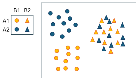
Fig. 6.3. Schematic diagram of a two-way crossed design where there is an interaction between factor A (with levels: A1 = blue and A2 = orange) and factor B (with levels: B1 = circles and B2 = triangles), demonstrating how interpreting the results of a test for differences in 'dispersion' of a main effect (e.g., factor B here) can be confounded by interactive effects of another factor (factor A here) on the centroids.
Clearly, if we did a PERMDISP test to compare the dispersions of the 2 groups corresponding to factor B (i.e., circles vs triangles), the result would be statistically significant. The graphic (Fig. 6.3) clearly shows that if you ignore factor A (i.e., if you ignore the colour of the symbols), then the circles are more spread out (dispersed) than the triangles. However, this actually has nothing to do with differences in 'dispersion' at all (all 4 of the A $\times$ B cells have roughly equal spread), but rather is due to the significant interaction in centroid effects. Specifically, at location B1 (circles) we see a shift in centroid due to factor A (A1 $\ne$ A2), but at location B2 (triangles), we do not see a shift in centroid due to factor A (A1 $\approx$ A2).
Continuing onwards now with our logical flow... If the test of (2) above is significant, then we effectively proceed with interpreting all of the results given in the PERMANOVA, including possibly doing relevant pairwise comparisons and associated ordination plots, etc.
If the test in (2) above is not significant, then we might consider doing the following two tests:
- (3) Test H03: dispersions of replicates within groups defined by factor A (ignoring factor B) are equal.
- Do a PERMDISP test to compare dispersions among levels of factor 'A'.
- (4) Test H04: dispersions of replicates within groups defined by factor B (ignoring factor A) are equal.
- Do a PERMDISP test to compare dispersions among levels of factor 'B'.
Depending on the outcomes of these tests (3) and (4), you could then do the two-factor PERMANOVA and account for heterogeneous dispersions in either of these factors, if needed.†
A few take-home messages
Handling potential heterogeneity of dispersions in multi-factor (PERM)ANOVA designs can potentially become very complex, as we have seen even in the two-way cases outlined above. However, it is important not to get too de-railed from the main game of your study, and there is no need to feel overwhelmed by this topic. Let's summarise a few take-home messages about all of this:
- PERMANOVA is very robust to heterogeneity if your design is balanced. If sample sizes are equal, you can use $F_1$ in the usual way for PERMANOVA and rest assured that the tests for centroid differences, interactions, etc. for all terms in the model generally will be quite robust and interpretable, regardless of any heterogeneity.
- If your design is unbalanced, test for heterogeneity in the highest-order cells and accommodate it. A useful standard approach for an unbalanced multi-factor design will always be to start by performing a PERMDISP on the highest-order cells in your study design. In other words, if you have 3 factors (A, B, and C), then create a factor that corresponds to all combinations of levels of those factors (A $\times$ B $\times$ C) and do a PERMDISP on that new 'combined' factor. If heterogeneity is present (among those cells), you can then easily accommodate it in your PERMANOVA by ticking the box to use $F_2$ ('Allow for heterogeneity') and nominating the highest order interaction term (e.g., A $\times$ B $\times$ C) in the PERMANOVA design file as the 'Term identifying groups with different dispersions'.
- Take one step at a time and think logically about each step in your testing procedure. If there is no heterogeneity in the dispersions of replicates among the highest-order cells in your study design, then you can proceed to examine a suite of logical hypotheses regarding differences in centroids and/or dispersions associated with other terms in your model. Usually, you would start with the higher-order terms in the model (towards the bottom of a PERMANOVA table of results) and gradually 'work your way up' towards considering the main effects. This might take some time and care, depending on the design and the number of simultaneous factors you are dealing with. Often, a helpful thing to think about is how the sum of squares (SS) for each term itself is constructed. This will point you to thinking about the right way to construct a test for homogeneity for any given factor or term in the model.‡ You will also have to consider how potential interactions (in centroid effects) among factors might alter your perception of dispersion differences across the main effects.
- If you have a (modestly) unbalanced design with (modest) heterogeneity, PERMANOVA is still quite a robust test. PERMANOVA is definitely focused on the null hypothesis of no differences in centroids. It is unlikely that modest differences in dispersion here or there are going to adversely affect your inferences drawn broadly from PERMANOVA tests much at all, especially if the degree of imbalance in your sample sizes is not dramatic (e.g., if you just have the odd replicate missing here or there in a few cells). Sometimes, the added complexity of dealing with heterogeneity (particularly if it occurs at multiple different levels and/or for more than one factor in your study design) can outweigh the benefits of attempting to accommodate it.
- Bear in mind that it takes quite a few replicates even to measure and compare dispersions in the first place. If you have very small sample sizes per cell (e.g., less than 4 or 5), then formal statistical comparisons of cell dispersions using PERMDISP are probably not worth much (i.e., they can be somewhat unreliable). Even in univariate analysis, you need far more replicates to get a decent estimate of the variance of a population than you would need to have in order to get a good estimate of the population mean. This is true also for multivariate dissimliarity-based analyses. So, if you have small sample sizes per cell, proceeding with the 'vanilla-flavoured' PERMANOVA (using $F_1$) to compare centroids (as you do not have much information even to estimate the dispersions for the cells) is quite a reasonable course of action.§
- Be cautious if you wish. If the design is unbalanced and the replication per cell is low, you can alternatively choose to take a more conservative stance: simply assume that there is heterogeneity among the cells, and do a PERMANOVA using $F_2$ accordingly. Taking that approach would be defensible, but perhaps would lack power.
¶ Note that adonis2 in the vegan package in R will not do any of this. Please see our recent exposé on this topic. In addition, no other software package that we know of (in R or otherwise) will implement PERMANOVA using $F_2$ or in any other way that accounts correctly for heterogeneity.
† In PRIMER 8 you can currently only specify one source of heterogeneity at a time in any given PERMANOVA model, although theoretically the general approach we use with $F_2$ need not be restricted necessarily in this way. It is only a matter of working out how to logistically accommodate multiple sources of heterogeneity simultaneously. Although this problem is not trivial, it is solvable. If you do have multiple sources of heterogeneity, then you will need potentially to consider running PERMANOVA more than once to account for this in the right way for tests of different terms in the model.
‡ For example, the SS for 'Locations' in the Nested design discussed on this page is constructed as the sum of squared deviations of 'Site' centroids around the 'Location' centroids. So that points us to: (i) first get the dissimilarities among the Site centroids, then (ii) do a PERMDISP for the location factor using those Site centroids as the 'replicates'.
§ Small sample sizes in cells may well have other consequences for your inferences, of course, such as limitations on the numbers of possible permutations for pairwise comparisons, thus limiting the precision of resulting p-values and, hence, low power.
6.8 Example: two-way crossed PERMANOVA allowing heterogeneity
We shall look at the diets of $N$ = 346 juvenile steelhead / rainbow trout (Oncorhynchus mykiss) obtained from 3 different rivers draining into Hood Canal, in the state of Washington, USA.¶ Some of the fish caught had been reared in a hatchery (identifiable by a clipped fin), and some were wild, of natural origin. Scientists studying these fish wanted to understand more about how the location (i.e., the river system) and the rearing of the fish (hatchery or wild-type) might affect the diets of these juvenile salmonid fish, both in terms of what they were eating on average (i.e., centroids) and how variable their diets were (i.e., dispersion).
The data file (named 'Hood_Canal_juv_salmonid_diets.pri', found inside the 'Examples_P8 > Hood_Canal_fish' folder) contains abundances of $p$ = 44 taxa found in the stomachs of individual fish (obtained by flushing). Note that each row of the file is an individual juvenile fish, and each column is a variable corresponding to items found in the stomachs of these fish (insects of various types, molluscs, etc.). The factor 'Hatchery' indicates whether the fish was hatchery-reared ('H') or wild type ('W'). The factor 'River' indicates which river system each fish was sampled from ('Dewatto', 'Duckabush', or 'Skokomish'). These data are unbalanced, as there is natural uncertainty regarding how many of the fish caught would end up being of hatchery origin. The number of replicates in each cell of the 2-factor crossed design is shown in Table 6.1 below.
Table. 6.1. Sample sizes ($n_{ij}$) in each of the 3 $\times$ 2 = 6 cells of the 2-factor crossed study design examining salmonid diets from Hood canal.
| Dewatto | Duckabush | Skokomish | Total | |
|---|---|---|---|---|
| Wild | 61 | 114 | 103 | 278 |
| Hatchery-reared | 35 | 22 | 11 | 68 |
| Total | 96 | 136 | 114 | 346 |
Pre-treat data, then calculate resemblances
- Open data in PRIMER - Start by opening the file in PRIMER by clicking File > Open... and navigating to the file named 'Hood_Canal_juv_salmonid_diets.pri'.
![14.Data_salmon_diets[i].png](https://learninghub.primer-e.com/uploads/images/gallery/2025-12/14-data-salmon-diets-i.png)
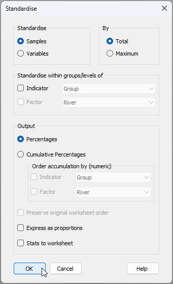
- Standardise data - We first need to standardise the data by total sample abundances (rows) to account for the fact that individual fish are different sizes and naturally would have had a different volume of prey in their stomachs at the time each one was caught. Click Pre-treatment > Standardise... > (Standardise: $\bullet$Samples) & (By: $\bullet$Total) & (Output: $\bullet$Percentages), then click 'OK'. The resulting sheet of standardised data will be called 'Data1'.
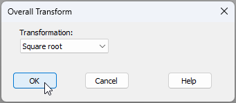
- Transform data - From the standardised data ('Data1' in the Explorer tree), apply a square-root transformation by clicking Pre-treatment > Transform(overall).... Choose Transformation: Square root, then click 'OK'. This will create a data sheet of standardised and transformed data called 'Data2'.
- Calculate resemblances - From the standardised and transformed data ('Data2' in the Explorer tree), calculate Bray-Curtis resemblances among all pairs of individual fish by clicking Analyse > Resemblance..., then choose (Measure $\bullet$Bray-Curtis similarity) & (Analyse between $\bullet$Samples), and click 'OK'.
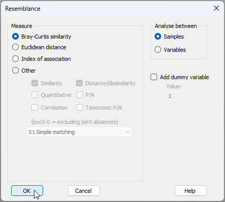
The resulting Bray-Curtis resemblances will be shown in the item named 'Resem1' in the Explorer tree, as shown below:
![18.Resem_matrix_salmonid_diets[i].png](https://learninghub.primer-e.com/uploads/images/gallery/2025-12/18-resem-matrix-salmonid-diets-i.png)
Test for homogeneity of dispersions across the cells of the 2-way design
Let's test for heterogeneity of dispersions among the cells in this 2-way crossed design.
- Create a combined factor - First, create a combined factor consisting of all combinations of 'River' and 'Hatchery'. Click Edit > Factors, click on the button labeled Combine..., then click on the 'Factors...' button. Next, click on each of the factors of 'River' and 'Hatchery' in turn (shown in the 'Available:' column on the left), then click on '>' to move them over to the 'Include:' column on the right.
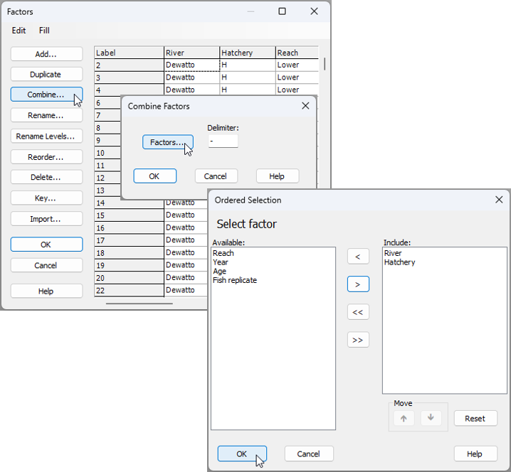
You will need to click 'OK' in both the 'Ordered Selection' dialog box, and also the 'Combine Factors' dialog box (as shown above), which will return you to the 'Factors' dialog box, where, if you scroll to the right, you should now see your newly created combined factor, called 'River-Hatchery' (see below):
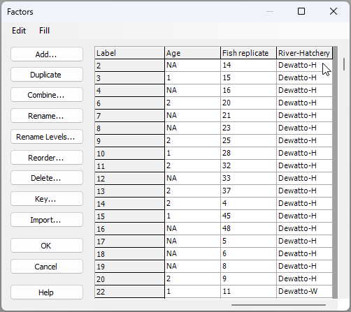
Click 'OK' and you are ready for the next step.
- Do a PERMDISP test - Let's do the test for homogeneity of multivariate dispersions across the cells corresponding to this combined factor. From the 'Resem1' matrix, click PERMANOVA+ > PERMDISP > (Group factor: River-Hatchery) & (P-values are from $\bullet$Permutation) & ($\checkmark$Do pairwise tests) & ($\checkmark$Output individual deviation values to worksheet).
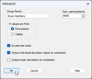
The output shows a highly significant result ($F_{5,340}$ = 16.535, $P$ = 0.0001), indicating there are highly significant differences in dispersion (variability in the diets) across these 6 cells.
![22.PERMDISP_output_salmonids[i].png](https://learninghub.primer-e.com/uploads/images/gallery/2025-12/22-permdisp-output-salmonids-i.png)
The mean distance-to-centroid values also show that for each river system, there is apparently greater dispersion (variability in diets) for the fish that were hatchery-reared, compared to the wild-type fish, on average; however, not all pairwise comparisons were statistically significant in this regard (e.g., for the Dewatto comparison of 'H' vs 'W', $t$ = 0.547 and $P$ > 0.50). Also provided in the output are the individual deviation values; that is, the distance to the cell centroid for each salmonid in the Bray-Curtis space. These are provided in the item named 'Data3' of the Explorer tree.
- Examine dispersion differences among cells - Let's create a means plot of the deviations from cell centroids as a useful way to visualise differences in dispersions (on average) across the cells. From the data sheet 'Data3', click Plots > Means Plot... > (Group factor: River-Hatchery) and untick the box in front of the words '$\square$Join means', then click 'OK'.
![23.Means_plot_salmonids_dialog[i].png](https://learninghub.primer-e.com/uploads/images/gallery/2025-12/23-means-plot-salmonids-dialog-i.png)
You should see the following plot ('Graph1'):
![24.Means_plot_deviates_salmonids[i].png](https://learninghub.primer-e.com/uploads/images/gallery/2025-12/24-means-plot-deviates-salmonids-i.png)
This plot suggests that the differences in the dispersions between the hatchery-reared and wild-type fish (with hatchery-reared fish being, on average, more variable in their diets) was greatest in the Skokomish river.
Test for equality of centroids, allowing for heterogeneous dispersions among cells.
Heterogeneity in dispersions among the cells of the study design is very clear and significant, and the number of replicates per cell is quite unbalanced; thus, we should run a two-way PERMANOVA examining the potential effects of river and hatchery-rearing on salmonid diets allowing for these differences in dispersions. We shall create an appropriate design file, then run the PERMANOVA analysis.
- Create a design file - From the 'Resem1' matrix, click PERMANOVA+ > Create PERMANOVA Design... to create an appropriate design file, as follows:
- Add a row by clicking on the button that says 'Add row' (
![Add_row_[i].png](data:image/png;base64,iVBORw0KGgoAAAANSUhEUgAAAF0AAAAXCAIAAADm0NSeAAAAAXNSR0IArs4c6QAAAARnQU1BAACxjwv8YQUAAAAJcEhZcwAADsMAAA7DAcdvqGQAAAASdEVYdFNvZnR3YXJlAEdyZWVuc2hvdF5VCAUAAAGHSURBVFhH7ZhLjoQgEIa5lgfiPJ7GzXS8gSakVqQOgMGwmDVmkgmCghSZlcRk8N9Y1sN0fV1lp2Hfr0pi/mKMkVICgGhYiGiMiVyMMQCwLMu2bT+tats2rTUAeDSOCyKu65onNimllJQycBFCWGvzlCZlrQWAyCWPNywhxMuloCe4YN91Pf7teVr1uGDfMVbsllKgnqdVjYtrlfNiu5QC9TytWlx8pwNPJmYfoCDvpZ6kuOeMMT5c0o7bWL57nOWN21SJy/HZI5iBh7bOIPUk1WcoSTs4DHy/OBic76GB3z1udbjEPg8waefepp5CObEDGM+VD35Q7h+XOlzS/QgrQlulnrS+GDq47Bw8nGDejaUKl7j3TmFi4ka5cNmTPCDe0j1yFu9CCvZumZLie1SBS/bln/27BvfxOX+mqKf4hOy9mz7zat6oClz+hV4uZUUuAPD+n/ay1kYuUkqlVJ7SpLTWiBi4+PM6rXXLU2OtVUpdzus8mnmeP5/PV6sax3Gapsv57iuqX7sIBlU6ePy1AAAAAElFTkSuQmCC) ), so there will be two rows in the design file, one for each factor in the design.
), so there will be two rows in the design file, one for each factor in the design. - In the first row, click in the blank cell in the first column and choose the factor of 'River', then in the second row, choose the factor of 'Hatchery'. These are both fixed and are crossed with one another, so no further changes to the design file are needed.
- Under the word 'Dispersions', tick the box that says '$\checkmark$Allow for heterogeneity' and click on the 'Groups' button. In the resulting pop-up box that says 'Select the term identifying groups with different dispersions' choose 'RiverxHatchery', then click 'OK'.
![Add_row_[i].png](https://learninghub.primer-e.com/uploads/images/gallery/2025-12/add-row-i.png)
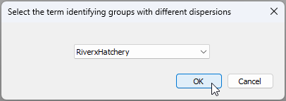
The resulting design file (called 'Design1') will look like this:
![25.PERMANOVA_2-way_design_Allow_het.disp_salmonids[i].png](https://learninghub.primer-e.com/uploads/images/gallery/2025-12/25-permanova-2-way-design-allow-het-disp-salmonids-i.png)
- Run a 2-way PERMANOVA (main test) - Now that we have the design file, we can run the PERMANOVA analysis. From the 'Resem1' matrix, click PERMANOVA+ > PERMANOVA.... Choose (Design worksheet: Design1) & (Action: $\bullet$Main test), with everything else in the dialog being left as the defaults, then click 'OK'.
![26.PERMANOVA_2-way_dialog_run[i].png](https://learninghub.primer-e.com/uploads/images/gallery/2025-12/ysC26-permanova-2-way-dialog-run-i.png)
The results of the analysis (in the item called 'PERMANOVA1' in the Explorer tree), show that there is a statistically significant interaction between the two factors of River and Hatchery in their effects on salmonid diets ($F_{2,44.21}$ = 4.20, $P$ = 0.0001).
![27.PERMANOVA_main_salmon[i].png](https://learninghub.primer-e.com/uploads/images/gallery/2025-12/27-permanova-main-salmon-i.png)
A casual glance at the expectations of the means squares and the construction of the $F$ statistics for each term in the model shows the complexity underlying these tests performed by the PERMANOVA routine.
![27b.PERMANOVA_main_salmon_EMS.etc[i].png](https://learninghub.primer-e.com/uploads/images/gallery/2025-12/27b-permanova-main-salmon-ems-etc-i.png)
It should also be noted, in passing, that we have used Type I SS here (sequential tests) and, as our sample sizes are unbalanced, the order in which we have chosen to fit these terms will matter to the results. We leave it up to the reader to consider re-running the analysis after changing the order of the factors (if desired) and/or to fit the PERMANOVA model using a different choice of sums of squares for the partitioning.
- Pair-wise tests - A natural next step, having observed a significant interaction, is to do pair-wise comparisons. We can consider two different sets of pair-wise comparisons that would each be of interest:
- (i) compare the diets for hatchery-reared fish vs wild-type fish separately within each river; and/or
- (ii) compare the diets for fish caught in different rivers (there will be three tests here: one for every pair of rivers) separately for each of the hatchery-reared fish and the wild-type fish.
The pair-wise tests can be done in a way that also allows for heterogeneity in dispersions. To pursue (i), from the resemblance matrix ('Resem1'), click PERMANOVA+ > PERMANOVA.... Choose (Design worksheet: Design1) & (Action: $\bullet$Pair-wise test > For term: RiverxHatchery > For pairs of levels of factor: Hatchery), with everything else being left as the defaults, then click 'OK'.
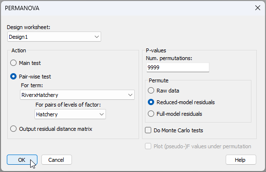
The results of these tests (i) are shown below in the output file 'PERMANOVA2'.
![30.Pairwise_results1[i].png](https://learninghub.primer-e.com/uploads/images/gallery/2025-12/30-pairwise-results1-i.png)
They show that, although there were no significant differences in the diets of hatchery-reared vs wild-type fish for the Dewatto river ($t_{68.67}$ = 1.107, $P$ > 0.25), there were differences between them detected in both the Duckabush ($t_{27.04}$ = 1.655, $P$ < 0.02) and Skokomish ($t_{11.24}$ = 2.67, $P$ < 0.001) river systems.
We can also do a set of tests comparing diets of fish in different rivers (ii) by repeating this procedure in precisely the same way, but choosing '(Action: $\bullet$Pair-wise test > For term: RiverxHatchery > For pairs of levels of factor: River)' in the PERMANOVA dialog instead (all else remaining the same). The results of those analyses are shown below ('PERMANOVA3'):
![30.Pairwise_results2[i].png](https://learninghub.primer-e.com/uploads/images/gallery/2025-12/30-pairwise-results2-i.png)
From this, we see that the diets of fish caught in each of the three rivers systems differed significantly from one another, whether they were hatchery-reared or wild-type fish (all pairwise tests had $P$ < 0.015).
Visualise centroid and dispersion differences
We may consider using a bootstrap average plot for a holistic view, along with ordinations of subsets of the data (e.g., corresponding to pair-wise tests), to elucidate differences in centroids and/or dispersions that may have been detected among cells in our study design. We shall demonstrate each of these with the salmonid dataset next.
- Holistic view: bootstrap averages - One useful way to visualise differences in centroids and in dispersions among cells simultaneously in a two-way (or multi-way) design such as this is to create a bootstrap average plot on the combined factor. Although the process of averaging bootstrapped data loses the details regarding inter-sample relationships among the original individual replicate sampling units, this type of plot does have the advantage of permitting a holistic view of the overall study and relationships among the cells in a single plot.
For the salmonid data set, begin at the resemblance matrix ('Resem1') and click Analyse > Bootstrap Averages... and choose (Factor: River-Hatchery), then in the 'MDS' section of the dialog, click on the 'MDS options...' button  . This will bring up a separate dialog box, and under 'Choice of intercept:' choose ($\bullet$ Threshold metric MDS (non-zero intercept)), then click 'OK' (you can leave the defaults for all the rest).†
![31.Bootstrap_average_salmonids_dialog_total[i].png](https://learninghub.primer-e.com/uploads/images/gallery/2025-12/31-bootstrap-average-salmonids-dialog-total-i.png)
The resulting bootstrap-average plot ('Graph2' in the Explorer tree), after a few alterations to symbols and colours‡, looks like this:
![32._Boot.av.plot_salmonids[i].png](https://learninghub.primer-e.com/uploads/images/gallery/2025-12/32-boot-av-plot-salmonids-i.png)
From this plot, we can see the following patterns, further supporting results of the statistical tests we have done:
- There is generally greater dispersion (variability) in the diets of hatchery-reared fish (light colours) compared to wild-type fish (dark colours).
- A difference between the diets of hatchery-reared fish vs wild-type fish (a shift in centroid) was detected for the Duckabush river (light red vs dark red) and the Skokomish river (light green vs dark green), but not for the Dewatto river (light blue vs dark blue).
- There were differences in the diets of fish caught from different river systems when we considered (separately) either the hatchery-reared fish (light green, light red and light blue are all distinct from one another), or the wild-type fish (dark green, dark red and dark blue are also all quite distinct from one another).
- The interaction between the factors is explained largely by the difference in the diets between hatchery-reared vs wild-type fish being much larger for fish caught in the Skokomish river than for those caught in the other river systems. For the Dewatto river, neither centroid nor dispersion effects were detected.
There are two important additional things to note about the above bootstrap average plot:
- First, the default colours and symbols in this bootstrap average plot produced by PRIMER 8 have been altered in the image above to make it easier to see changes in centroid and/or dispersion for the factors of interest.‡
- Second, we must not forget that every symbol on this plot is an average, and the dispersion of averages is therefore going to reflect not just the dispersion of the original data, but also the sample size. More specifically, we already should expect that the larger the sample size, the smaller the group's dispersion is expected to appear, due simply to the central limit theorem.§ For this reason, we must take observed differences in dispersion seen in a bootstrap average plot with a certain grain of salt when sample sizes differ among the groups (as here). Examining individual plots of dispersions of replicate sampling units (for subsets of the data, if necessary, as in step 12 below) will help to clarify the extent of genuine underlying dispersion differences among groups.
- Detailed view: ordinations of subsets - Another way to visualise various aspects of these results is to 'zoom in' and examine ordination plots of sub-sets of the full dataset, such as those corresponding to pair-wise tests. This is a bit more direct than the bootstrap average approach, permitting investigation of the original inter-sample relationships among replicates, but of course each plot is restricted in its focus to a particular sub-set of the data, so the 'big-picture' information about relationships among all of the cells in the study design (as seen in the bootstrap average plot) is not able to be seen.
For example, let's consider aiming to visualise the pair-wise results from tests done according to point 10(i) above. We need to split the data into three groups according to the three river sytems and run nMDS on each one, removing the labels and showing symbols for the factor 'Hatchery' on the resulting plots. You could start from the standardised and transformed data sheet (called 'Data2' in the Explorer tree) and click on Tools > Split Data... > (Samples > $\checkmark$Split by factor: River). Rename the resulting 3 datasheets according to the appropriate 3 river names, and proceed from there to calculate Bray-Curtis, then nMDS in each case. Doing this yields the following graphics:
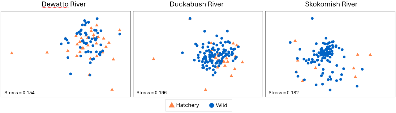
Relevant things to note about the above plots are:
- For the Duckabush river, there is no apparent difference between the diets of hatchery-reared vs wild-type fish in terms of either their centroids or their relative dispersions; this is in line with the non-significant test results for PERMDISP and PERMANOVA that were found (above) for this river.
- For the other two rivers (Duckabush and Skokomish), a shift in centroid and a change in dispersion is apparent in both nMDS plots, although the stress in both of these final 2D configurations is quite large (approaching 0.2). We should therefore refrain from making any further interpretations of fine-scale patterns.
A similar set of ordinations on sub-sets of data may also be constructed to help visualise pair-wise results from tests done according to point 10(ii) above. We shall leave it to the reader to consider examining those on their own, if desired.
¶Data courtesy of Katie Doctor-Shelby, formerly based at the Northwest Fisheries Science Centre, National Oceanic and Atmospheric Administration (NOAA), Seattle, WA, USA.
†Note: the default here is to calculate 50 bootstrap averages per group. This can take a long time to execute! You may wish to speed up the process by choosing to do just 25 or 30 bootstraps instead.
‡ If you click on the legend itself inside the bootstrap average plot, you will see a complete legend key, as shown below. To the left is the default legend in PRIMER 8, and to the right are the customised symbols and colours I chose for the example. I find that when I do a bootstrap average plot (or a plot of distances among centroids) where the 'averages' are actually 'cells' in a factorial design (as here, where we have 3 $\times$ 2 = 6 cells in a two-way crossed design), it is useful to create a colour and symbol scheme that will make it easy to compare levels of factors of interest. For example, in the present case, I used blue, red and green for the three different rivers, then chose a lighter tint for the hatchery-reared fish and a darker shade for the wild-type fish (see the 'customised' key on the right in the image below). I also used a common symbol for each river system as well (although one could use, say open vs closed symbols as another option here). However, if you wish to cater carefully for any type of colour-blindness, then you will find that the default colours now used in PRIMER 8 are designed especially to do this. You might also find that maintaining the use of different readily distinguishable symbols for all of the cells in the design is a good idea. For this example, see the default legend shown at left below, and the associated default bootstrap average plot below that.
![33.Key_comparison_salmonids_both[i].png](https://learninghub.primer-e.com/uploads/images/gallery/2025-12/33-key-comparison-salmonids-both-i.png)
![34._Boot.av.plot_salmonids_default_colours[i].png](https://learninghub.primer-e.com/uploads/images/gallery/2025-12/34-boot-av-plot-salmonids-default-colours-i.png)
§Recall the central limit theorem from classical univariate statistics. Let $Y$ be a random variable with an unknown distribution that has a mean of $\mu_Y$ and a variance of $\sigma_Y^2$. Now suppose you take a random sample of size $n$ with realised values $\lbrace y_1, y_2, \ldots, y_n \rbrace$ and calculate the average of that sample as: $\bar{y} = \sum_{i=1}^n y_i$. This average is then a random representative of variable $\bar{Y}$, which has a distribution that converges to a normal distribution, with a mean of $\mu_Y = \mu_{\bar{Y}}$ and a variance of $\sigma_{\bar{Y}}^2 = \sigma_Y^2/n$. Thus, it is clear that the distribution of the averages has a variance that gets smaller and smaller, the greater the sample size. Similarly, we expect the dispersion of averages (whether bootstrapped or otherwise) for a group of multivariate sampling units will get smaller and smaller (all else being equal) the larger the sample size of that group.